Open Journal of Soil Science
Vol.1 No.2(2011), Article ID:7585,8 pages DOI:10.4236/ojss.2011.12003
Experimental and Modeling Investigation of Shallow Water Table Fluctuations in Relation to Reverse Wieringermeer Effect
![]()
Graduate School of Agricultural and Life Sciences, The University of Tokyo, Tokyo, Japan.
Email: *ibrahimi@soil.en.a.u-tokyo.ac.jp
Received June 14th, 2011; revised July 20th, 2011; accepted August 8th, 2011.
Keywords: Groundwater Fluctuation, Shallow Water Table, Reverse Wieringermeer Effect, Capillary Fringe
ABSTRACT
Soil column experiments and modeling investigations were performed to study the behavior of shallow water table in response to various recharge events. Hence, shallow water table fluctuations inside sandy (Toyoura sand) and clayey (Chiba light clay) soil columns in response to surface and sub-surface recharge events were investigated under laboratory conditions. Experimental results showed that small application of water could raise the shallow water table level more than 100 times in depth in the case of Toyoura sand and more than 50 times in the case of Chiba LiC, reflecting a reverse Wieringermeer effect (RWE) response type of groundwater. This rise was associated with a prompt change of pressure head values which exhibited instantaneous fluctuations of centimeters due to the addition of millimeters of water. The recharge volumes leading to such disproportionate water table rise were successfully estimated using a simple analytical model based on the moisture retention curve of the soil and considering the hysteresis effect on soil water dynamics within the capillary fringe zone.
1. Introduction
Shallow groundwater systems (SGS) are important as a source of water, for sustenance of stream base flow and of wetland and riparian ecosystems [1]. They have been recognized to have effects on a broad variety of earth system processes [2,3]. Accordingly, the proper management of these valuable groundwater resources requires an accurate quantification of their recharge rates. Such quantification is not easy to handle due to the dynamic nature of these systems having a very fast response time to hydrologic change owing to their closeness to soil surface [1]. In fact, many researchers reported rapid and disproportionate water table rise in response to rainfall events observed in shallow groundwater systems [4-6]. They showed that shallow water tables can often rise disproportionately compared to the volume of infiltrated water. This rise has been attributed by numerous researchers to one of two major phenomena. The first, known as the Lisse effect, occurs when infiltration caused by intense rain seals the surface soil layer to airflow, trapping and compressing air under pressure in the unsaturated zone [7,8]. For a comprehensive outline of the Lisse effect, the reader is referred to [8]. The second is the reverse Wieringermeer effect (RWE) dealing with the case where the capillary fringe extends from the water table almost to the ground surface leading to a limited or no storage capacity in the zone between water table and soil surface as well as a specific yield approaching zero value. In these conditions the pores within the capillary fringe are saturated and the addition of a very small amount of water relieves the tensions in the capillaries resulting in a rapid and high water table rise to the land surface [9,10]. The specific yield was defined as the volume of water that an aquifer releases from storage per unit surface area of aquifer per unit decline in the water table [11].
It was demonstrated through numerical studies and laboratory as well as field investigations that, under RWE conditions, the estimation of water table responses to recharge events based on the maximum or ultimate specific yield, which can be estimated from an equilibrium soil water profile, is erroneous and always underestimates the rate and total amount of water table rise [12, 13]. Gillham [9] pointed out that the shallow water table response to added water could be explained by considering the specific yield above a shallow water table to be variable, with values decreasing as the water table approaches ground surface.
In view of the facts mentioned above, the aim of this work is threefold: 1) to investigate experimentally shallow groundwater responses to surface and sub-surface recharge events using two soil types (sandy and clayey), 2) to verify the applicability of RWE concept under these experimental conditions, 3) to develop a quantitative analysis based on hysteresis model in order to simulate the experimental results.
2. Theoretical Background
Figure 1 depicts the hypothetical moisture profiles above a rising deep water table (WT1) and shallow water table (WT2). These profiles are represented by the moisture retention curve of the soil with the assumption that static equilibrium conditions prevailed. After a change of water level, the water table WT1, which was initially at depth d, will rise by dh to a new level d′. It is assumed that the static equilibrium profile is re-attained instantaneously. Further, the flow is assumed to be one-dimensional and no water flux at the bottom boundary. In these conditions, the dotted area A representing the volume of water per unit area that is added to storage due to the water-level rise from d to d′ is equal to Sydh, where Sy is the specific yield of the soil.
Consider now the case of a shallow water table WT2 being initially at the level d″. This depth is not great enough to allow moisture content at land surface to reach the value of residual moisture content. In this case, the dotted area A representing the water yield is less than Sydh (Figure 1). The discrepancy between actual yield and that calculated on knowledge of Sy and dh has been observed to increase as depth to water table decreases [9, 11,12]. This phenomenon, referred to as the reverse Wieringermeer effect, is reflected by a nearly instantaneous rise in water level in response to only a small amount of infiltration.
The dotted area A can be mathematically expressed as:
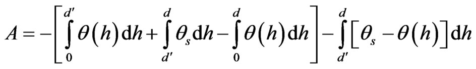 (1)
(1)
where θs is saturated water content and θ(h) is the water content-pressure head relationship. The minus sign is used to account for the negative pressure head.
The van Genuchten model (hereafter VG) of water retention relationship [14] was used in the present study to describe the boundary drying and wetting curves. This model assumes that the main drying and wetting retention curves can be described accurately by the expression:
 (2)
(2)
where θr is residual water content, α, m, n are fitting parameters, with m = 1 – 1/n. Replacing Equation (2) in Equation (1) yields:
 (3)
(3)
In order to account for hysteresis effect, we assume that between the initial water table level d and the final depth d’, the groundwater will follow a scanning wetting curve starting from a preceding drying curve (reversal point). Scanning curves can be determined experimentally by a series of wetting and drying experiments. Such measurements are extremely time-consuming and delicate to carry out. Therefore, a theory is needed to estimate the water-retention function for any drying and wetting loop based on the envelope of main drying and wetting curves. Numerous models have been developed in order to describe the hysteretic behavior of a particular soil [15-18]. In the present study we used the modified Kool and Parker model [17] developed by Huang et al. [18]. This model of simple formulation uses α, n, θsd = θsw and θrd = θrw as variables (d and w denote for drying and wetting, respectively). Additionally, αw, nw and αd, nd are assigned the same values in describing various wetting and drying scanning curves. In this model, the relationship of θ (h) for the ith-order scanning curve with no pumping effect can be obtained using θsw(i) and θrw(i) or θsd(i) and θrd (i). Hence, once θs(i) and θr(i) are defined, Equation (3) is integrated numerically using the trapezoidal rule of integration in order to estimate the water supply amount AH (H for hysteresis) between water table depths d and d′. Equation (3) becomes:
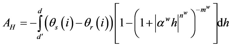 (4)
(4)
where θs(i) and θr(i) are saturated and residual water contents, respectively, corresponding to the ith-order scanning curve, αw, nw, mw are fitting parameters and h pressure head.
3. Material and Methods
3.1. Soil Column and Measurement System Set up
Soils of two textures were used for this research: i) Toy-
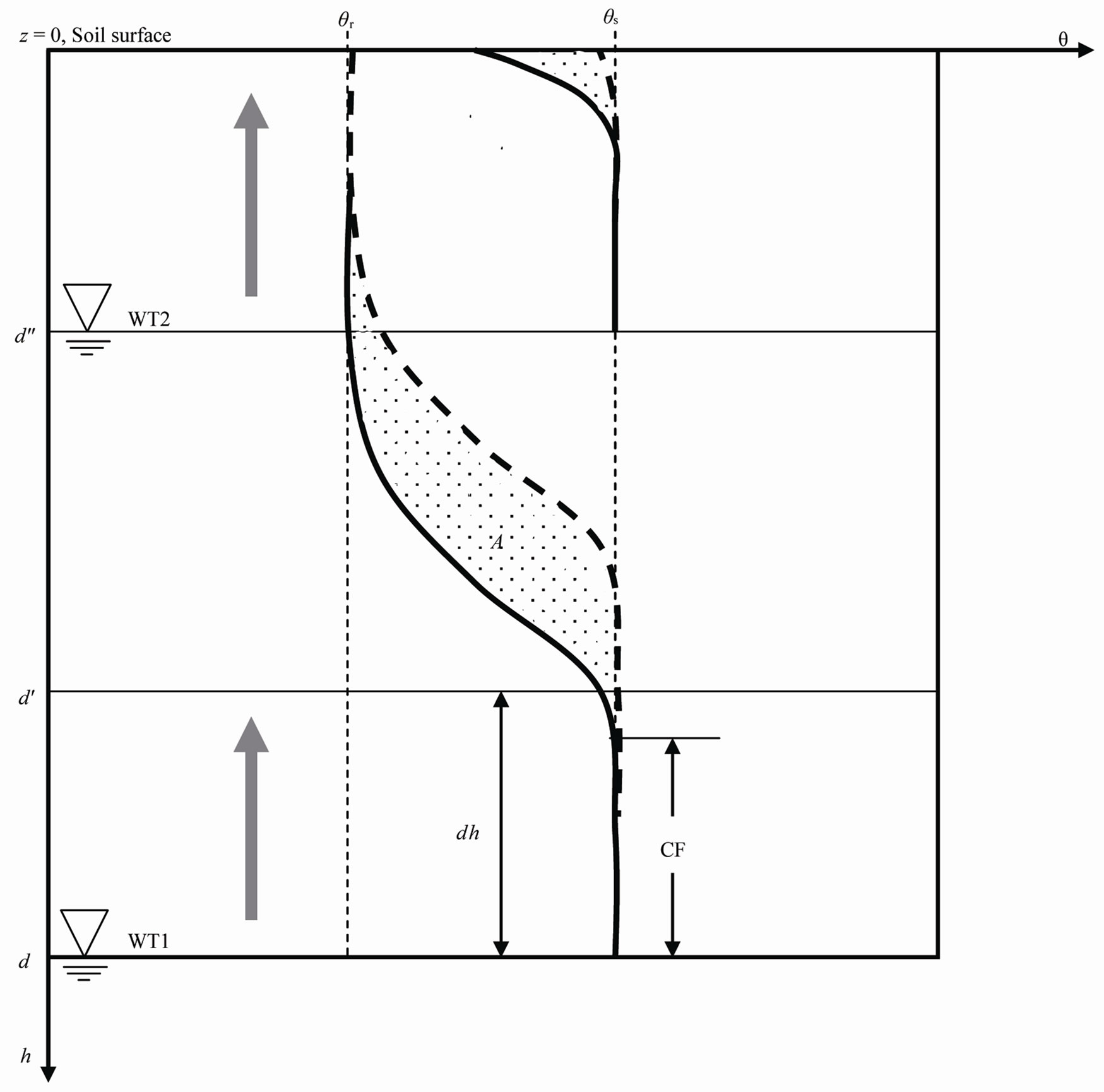
Figure 1. Conceptualized moisture profiles above a deep water table (WT1) and a shallow water table (WT2). CF: capillary fringe; A: water recharge; θr: residual water content; θs: saturated water content (adapted from Healy and Cook [11]).
oura sand from Toyoura, Yamaguchi, Japan, having a grain size ranges between 0.02 mm to 0.30 mm with a mean value of 0.125 mm, and ii) Chiba light clay (Chiba LiC) collected at a depth of 80 cm in an experimental farm at Chiba Prefectural, Agricultural and Forestry Research Center. Particle-size analyses for the Chiba LiC soil showed percentage distributions of 52.8/20.7/26.5 for sand/silt/clay, respectively.
In the present study, laboratory measurements of θ(h) in the drying and wetting processes for Toyoura sand and Chiba LiC were carried out using the hanging method [19]. The measurements of drying and wetting curves were done separately on different soil samples. In relevance to our experimental conditions, described above, we restricted our analysis in the range of pressure 0 - 100 cm H2O. The experimental data were then fitted using the VG model. Figure 2 shows both measured and simulated data of the main water retention curves of Toyoura sand and Chiba LiC. It can be seen clearly that the two pathways (i.e. drying and wetting) produce curves that are not identical. The water content in the drying curve is higher for a given matric potential than that in the wetting branch depicting the hysteretic nature of both soils. The VG model fitted fairly well (R2 = 0.99) the observed main wetting and drying curves in the case of Toyoura sand and Chiba LiC soils. The θ(h) curves are useful to estimate the height of the capillary fringe defined as the region between h = 0 and h = ha where ha is the pressure

Figure 2. Water retention curves of Toyoura sand and Chiba light clay.
head at which the first pore drains. Hence, Figure 2 shows that for Chiba LiC soil, the capillary fringe extends, in the drying process, to approximately 15 cm while in the case of Toyoura sand this zone extends to almost 40 cm above the water table level.
Toyoura sand and Chiba LiC soils were packed homogenously into two acrylic columns with 50 cm length and 7.5 cm inner diameter. The Toyoura sand column was equipped with 17 acrylic resin porous cups along the profile (Figure 3). The Chiba soil column was equipped with 11 ceramic porous cups made of very thin, small and sensitive ceramics in order to insure a reasonably rapid response time. In both columns, the porous cups were connected to a series of pressure transducers with a 0 to 100 kPa range, for continuous measurement of pressure head at each of the monitoring locations. The water table level was monitored by means of a water manometer. Two Mariotte tubes with 5 cm and 0.7 cm inner diameters have been used for soil saturation process and for water recharge from the bottom side of the column, respectively.
3.2. Experimental Procedure
Two experiments (Exp 1 and Exp 2) have been conducted using Toyoura sand and Chiba light clay, respect-

Figure 3. Schematic diagram of the laboratory experimental apparatus.
tively. The Exp 1 consisted of performing the total of four experimental runs numbered 1 through 4. During the runs 1 and 2, water table was positioned initially at 20 cm and 40 cm, respectively, by using a drip point. Then, various amounts of water have been added from the top side of the soil column, as simulated rainfall events (surface recharge). The hydrostatic condition in the entire soil column after each rainfall event formed the initial condition for the subsequent water supply. During the runs 3 and 4, water was supplied from the bottom (subsurface recharge). In the Exp 2, the total of six experimental runs numbered 5 through 10, have been carried out. Almost, the same procedure used in Exp 1 was reproduced in Exp 2 during which water table was set initially at 15 cm, 30 cm and 70 cm depths.
4. Results and Discussion
4.1. Water Table Fluctuations in Response to Recharge Events
In all experimental runs during the experiments 1 and 2, the water table rise after each water supply event was isolated and plotted against water applied amount (Figure 4). Linear trend lines have been fitted to each of the experimental runs and regression equations have been developed.
In all experimental runs, recharge events and their water table responses exhibited a linear relationship of the form: WTL = a·R, where WTL (cm) is the water table level, a (dimensionless) is a regression coefficient and R (cm) is the recharge amount. In the case of Toyoura sand, the regression equation developed from the water table response during the experimental run 1, shows that the addition of 1 mm water as a rainfall event brought about
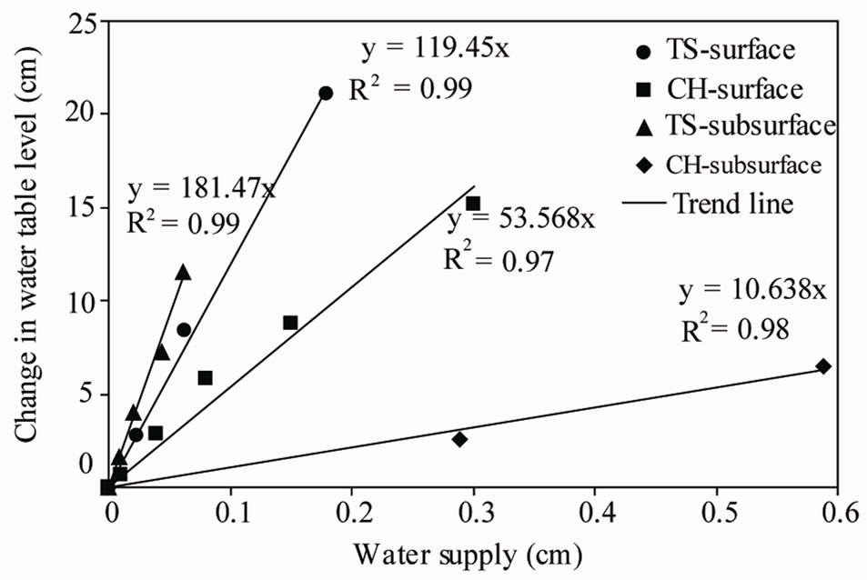
Figure 4. Correlations between cumulative added water events as surface and sub-surface recharge and the corresponding change in water table level in the case of Toyoura sand (WT at 20 cm) and Chiba LiC (WT at 15 cm) soils. TS: Toyoura sand; CH: Chiba LiC.
120 mm water table rise for initial water table position at 20 cm depth, reflecting a reverse Wieringermeer response type. Considering the specific yield of Toyoura sand used in this experiment of 0.3 [20], multiplied by the water table rise of 120 mm would result in 36 mm of recharge water compared with the 1 mm of simulated rain that actually has been added during the run 1. This shows that the specific yield method gives erroneous estimates of recharge if used under RWE conditions.
Similar to the case of Toyoura sand, the water table increase during Chiba LiC experiment was also highly correlated to rainfall in all experimental runs (R2 ³ 0.97). Compared to Toyoura sand, the water table rise in Chiba LiC experiment was less pronounced suggesting the soil type effect on groundwater response. With respect to water table responses to sub-surface recharge events, it can be seen, as shown in Figure 4, that in the case of Toyoura sand, sub-surface recharge caused a disproportionate water table rise. In the case of Chiba LiC, the water table increased linearly in response to sub-surface water input, with remarkably a lower magnitude than that observed for Toyoura sand.
4.2. Pressure Head Responses to Recharge Events
Figure 5 illustrates the pressure head profiles at several times across Toyoura sand and Chiba LiC columns, for
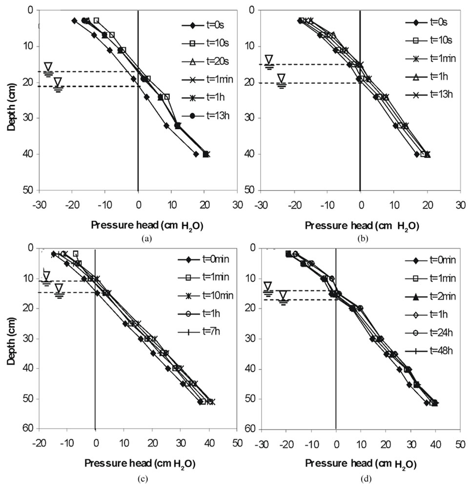
Figure 5. Pressure head versus depth profiles showing the elevation of the water table in the case of Toyoura sand (surface (a), sub-surface (b)) and Chiba LiC (surface (c), sub-surface (d)).
water table initial levels at 20 cm and 15 cm, respectively. The time t = 0 represents the initial condition before water application. It can be seen that the response was evident at all measuring points immediately following the initial application of recharge events. Pressure head values exhibited instantaneous fluctuations of centimeters due to the addition of millimeters of water. Being the locus of points having zero pressure head, the position of the water table could be, in principle, determined at any time by interpolating or extrapolating the pressure head values [21]. This approach is used in order to monitor the water table elevation.
In the case of Toyoura sand, we observed a rapid and high water table rise immediately after water supply from the top side of soil column (Figure 5(a)). In fact, after the application of 1 mm rainfall water table rose, within the first 10 seconds, by 5 cm. Following this rise there was a relatively rapid decline. This decline can be explained by the fact that as the rise is caused by the change in the pressure potential in capillary fringe from negative to positive values due to the addition of a small amount of water, the water table declines very quickly with the loss of a small amount of water by downward drainage. When water was added by sub-surface recharge, a rapid change in pressure head was observed although less pronounced compared to that observed for surface recharge mode (Figure 5(b)).
The pressure head profiles in the case of Chiba LiC soil showed that water table manifested a slower response compared to Toyoura sand (Figure 5(c) and (d). Thus, when water table was set initially at 15 cm below soil surface, it rose by approximately 3 cm after 20 seconds have passed. In the case of sub-surface recharge, addition of water resulted in a gradual water table rise.
4.3. Discussion and Modeling Investigation
From the aforementioned experimental results two important questions arise: 1) Why the same recharge volume brought about different water table responses when applied by surface and sub-surface recharge modes? 2) What caused the difference of water table behavior between the two soil types, Toyoura sand and Chiba LiC?
In the present study, we are dealing with the water table rise from bottom to soil surface. In our experiments, the initial moisture content is low at the soil surface and getting higher toward the bottom, leading to higher propagation velocity of pressure wave. Under these conditions, the experimental results showed that sub-surface water supply caused a higher water table rise compared to surface recharge mode. This is most likely induced by larger water flux at the soil bottom (saturated) due to larger hydraulic conductivity, than at the top of the soil profile. Further, when the capillary fringe extends to soil surface, the initial water content above water table is close to saturation which causes a small amount of added water to produce a large rise of the water table.
It is widely accepted that groundwater response to recharge events is related to the shape of the soil moisture profile above the water table and its potential significance is determined by the water content-pressure head relation (WRC) of the soil [9]. Since this relation is unique for each soil type, the groundwater response is variable from one soil type to another.
In order to investigate the validity of this concept to explain the observed groundwater behavior in our experiments we adopted a simple modeling approach based on a parameterization of saturated and residual volumetric water contents by considering the hysteretic behavior of the water retention curve. In this approach we assumed that the soil moisture profile changes from an initial hydrostatic condition to a new one following water table rise. The change of water table level is induced by water supply either by surface or sub-surface recharge. Moreover, since the soil water movement is upward due to groundwater rise, the soil moisture profile is most likely described by the wetting moisture retention curve.
For the purpose of comparison we also investigated a modeling approach based on the wetting process of the water retention curve and considering the range of moisture content in the zone above water table between saturated  and residual
  water content of the wetting moisture curve. The recharge is denoted AW, (W for wetting). The water recharge amount AW is estimated by integrating the following equation:
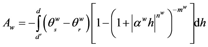 (5)
(5)
Figures 6 and 7 depict the results of model predictions and measurements of water supply events and their corresponding changes in water table level for Toyoura sand and Chiba LiC soils, respectively. It can be seen that the simulations based on the wetting curve parameters (AW) gave a very poor prediction. In fact, the model AW always underestimated the groundwater fluctuations. By considering hysteresis effect, the predictions of recharge volumes were improved. Hence, a very good agreement between measured and estimated water recharge volumes is obtained with the model AH. Interestingly, we see that the simulation based on this model succeeded in predicting general features of the water table fluctuations in most of the experimental tests. This suggests that the soil water movement inside the soil column is mainly upward from the lower part being wetting up after water supply.

Figure 6. Measured and simulated recharge amounts and their corresponding changes in water table levels for Toyoura sand. AH, AW: simulated data using (4) and (5) respectively; WTi: initial water table depth.

Figure 7. Measured and simulated recharge amounts and their corresponding changes in water table levels for Chiba LiC. AH, AW: simulated data using (4) and (5) respectively; WTi: initial water table depth.
Further, these results indicate that the shallow ground water had a great effect on the vertical distribution of soil.
5. Conclusions
In the present study, laboratory simulations of shallow groundwater fluctuations in response to surface and subsurface recharge events showed that both recharge modes can cause water table fluctuations. Hence, for both cases, groundwater exhibited a reverse Wieringermeer response type to water input reflected by a rapid and large water table rise in response to a small volume of added water. This was substantiated by the pressure head responses following water application. In fact, when groundwater was set at shallow depths most changes were observed immediately following water application either from the top or bottom side of the soil column.
There were major differences, however, in groundwater behavior depending on the water table initial depth, the soil type and the way of water input. Thus, in the case of Toyoura sand, water table rose by hundred times the depth of added water while in the case of Chiba light clay, water table rise was less pronounced and slower.
A proposed water table response model based on soil moisture retention curve and considering the hysteresis effect gave good fit with experimental measurements. These simulations showed that water content profiles are dependent on the preceding sequence of wetting and drying and suggest the importance of including hysteresis in numerical simulation of systems undergoing reverse Wieringermeer effect leading to cyclic soil moisture changes.
6. Acknowledgements
The doctoral research scholarship provided to the first author by the Tunisian Government is thankfully acknowledged. The authors would like also to express their gratitude to Dr. Arihara from Chiba Prefectural, Agricultural and Forestry Research Center for his permission and assistance in collecting Chiba light clay soil.
REFERENCES
- P. Dillon and I. Simmers, “Shallow Groundwater Systems: IAH International Contribution to Hydrogeology 18,” Taylor and Francis, Rotterdam, 1998.
- S.W. Tyler, J. F. Munoz and W.W. Wood, “The Response of Playa and Sabkha Hydraulics and Mineralogy to Climate Forcing,” Ground Water, Vol. 44, 2006, pp. 329-338. doi:10.1111/j.1745-6584.2005.00096.x
- L. Xu, J. Yang, Q. Zhang and H. Niu, “Modelling Water and Salt Transport in a Soil-Water-Plant System under Different Groundwater Tables,” Water and Environment Journal, Vol. 22, 2008, pp. 265-273. doi:10.1111/j.1747-6593.2007.00102.x
- A. L. O'Brien, “Rapid Water Table Rise,” Journal of the American Water Resources Association, Vol. 18, No. 4, 1982, pp. 713-715. doi:10.1111/j.1752-1688.1982.tb00056.x
- N. Cartwright, T. E. Baldock, P. Nielsen, D. S. Jeng and L. Tao, “Swash-aquifer Interaction in the Vicinity of the Water Table Exit Point on a Sandy Beach,” Journal of Geophysical Research, Vol. 111, 2006, pp. 1-13. doi:10.1029/2005JC003149
- K. Ibrahimi, T. Miyazaki and T. Nishimura, “A High Measurement Frequency Based Assessment of Shallow Groundwater Fluctuations in Metouia Oasis, South Tunisia,” Hydrological Research Letters, Vol. 4, pp. 75-79. doi:10.3178/HRL.4.75
- F. D. Heliotis and C. B. DeWitt, “Rapid Water Table Responses to Rainfall in a Northern Peatland Ecosystem,” Water Resources Bulletin, Vol. 23, 1987, pp. 1011-1016.
- E. P. Weeks, “The Lisse Effect Revisited,” Ground Water, Vol. 40, 2002, pp. 652-656. doi:10.1111/j.1745-6584.2002.tb02552.x
- R. W. Gillham, “The Capillary Fringe and its Effect on Water Table Response,” Journal of Hydrology, Vol. 67, No.1-4, 1984, pp. 307-324. doi:10.1016/0022-1694(84)90248-8
- D. P. Horn, “Measurements and Modeling of Beach Groundwater Flow in the Swash-Zone: A Review,” Continental Shelf Research, Vol. 26, No. 5, 2006, pp. 622- 652. doi:10.1016/j.csr.2006.02.001
- R. W. Healy and P. G. Cook, “Using Groundwater Levels to Estimate Recharge,” Hydrogeology Journal, Vol. 10, No. 1, 2002, pp. 91-109. doi:10.1007/s10040-001-0178-0
- M. Sophocleous, “The Role of Specific Yield in Groundwater Recharge Estimations: A Numerical Study,” Ground Water, Vol. 23, No. 1, 1985, pp. 52-58. doi:10.1111/j.1745-6584.1985.tb02779.x
- F. H. Jaber, S. Shukla, and S. Srivastava, “Recharge, Upflux and Water Table Response for Shallow Water Table Conditions in SE Florida,” Hydrological Processes, Vol. 20, No. 9, 2006, pp. 1895-1907. doi:10.1002/hyp.5951
- M. T. van Genuchten, “A Close-Form Equation for Predicting the Hydraulic Conductivity of Unsaturated Soils,” Soil Science Society of America Journal, Vol. 44, No. 5, 1980, pp. 892-898. doi:10.2136/sssaj1980.03615995004400050002x
- Y. Mualem, “A Conceptual Model of Hysteresis,” Water Resources Research, Vol. 10, No. 3, 1974, pp. 514-520. doi:10.1029/WR010i003p00514
- Y. Mualem and G. Dagan, “A Dependence Domain Model of Capillary Hysteresis,” Water Resources Research, Vol. 11, No. 3, 1975, pp. 452-460. doi:10.1029/WR011i003p00452
- J. B. Kool and J. C. Parker, “Development and Evaluation of Closed-Form Expressions for Hysteretic Soil Hydraulic Properties,” Water Resources Research, Vol. 23, No. 1, 1987, pp. 105-114. doi:10.1029/WR023i001p00105
- H. C. Huang, Y. C. Tan, C. W. Liu and C. H. Chen, “A Novel Hysteresis Model in Unsaturated Soil,” Hydrological Processes, Vol. 19, No. 8, 2005 pp. 1653-1665. doi:10.1002/hyp.5594
- A. Klute, “Water Retention: Laboratory Methods. Methods of Soil Analysis. Part 1 Physical and Mineralogical Methods,” 2nd Edition, American Society of Agronomy, New York, 1986, pp. 635-662.
- M. Price, “Specific Yield Determinations from a Consolidated Sand Stone Aquifer,” Journal of Hydrology, Vol. 33, No. 1-2, 1977, pp. 147-156. doi:10.1016/0022-1694(77)90104-4
- A. S. Abdul and R. W. Gillham, “Laboratory Studies of the Effects of the Capillary Fringe on Stream Flow Generation,” Water Resources Research, Vol. 20, No. 6, 1984, pp. 691-698. doi:10.1029/WR020i006p00691