Open Journal of Modern Hydrology
Vol.07 No.02(2017), Article ID:74751,25 pages
10.4236/ojmh.2017.72004
Assessing the Hydrology of a Data-Scarce Tropical Watershed Using the Soil and Water Assessment Tool: Case of the Little Ruaha River Watershed in Iringa, Tanzania
Winfred B. Mbungu1*, Japhet J. Kashaigili2
1Department of Engineering Sciences and Technology, Sokoine University of Agriculture, Morogoro, Tanzania
2Department of Forest Resources Assessment and Management, College of Forestry, Wildlife and Tourism, Sokoine University of Agriculture, Morogoro, Tanzania
![]()
Copyright © 2017 by author(s) and Scientific Research Publishing Inc.
This work is licensed under the Creative Commons Attribution International License (CC BY 4.0).
http://creativecommons.org/licenses/by/4.0/


Received: December 23, 2016; Accepted: March 13, 2017; Published: March 16, 2017
ABSTRACT
The hydrology of the Little Ruaha River which is a major catchment of the Ihemi Cluster in the Southern Agricultural Growth Corridor of Tanzania (SA- GCOT) has been studied. The study focused on the hydrological assessment through analysis of the available data and developing a model that could be used for assessing impacts of environmental change. Pressures on land and water resources in the watershed are increasing mainly as a result of human activities, and understanding the hydrological regime is deemed necessary. In this study, modeling was conducted using the Soil and Water Assessment Tool (SWAT) in which meteorological and streamflow data were used in the simulation, calibration and evaluation. Calibration and evaluation was done at three gauging stations and the results were deemed plausible with NSE ranging between 0.64 and 0.80 for the two stages. The simulated flows were used for gap filling the missing data and generation of complete daily time series of streamflow at three gauging stations of Makalala, Ihimbu and Mawande. Results of statistical trends and flow duration curves, revealed decline in magnitudes of seasonal and annual flows indicating that streamflows are changing with time and may have implications on envisioned development and the water dependent ecosystems.
Keywords:
Hydrology, Little Ruaha, Anthropogenic Activities, SWAT-CUP

1. Introduction
Freshwater ecosystems are vital and crucial limited resources to the survival of human beings as well as for sustaining ecosystems around the globe. Apart from sustaining the environment and conservation, freshwater ecosystems provide services for socio-economic, supporting such activities as irrigation, energy supply and directly impact human livelihoods [1] [2] . However, despite their value and importance, freshwater ecosystems around the world are being threatened by the increase in anthropogenic activities as a result of pressure from increased population growth [1] [3] [4] .
In recent decades, the challenge of feeding the world population has increased demands for increasing food production, and hence expansion of croplands. Approximately 38% of the global land surface are occupied by croplands and grazing lands [5] [6] [7] . According to the World Bank [8] , agriculture employs more than 31% of the world population. This number is even higher for developing countries like Tanzania where over 75% of the population is directly dependent on agriculture [9] [10] . Various studies have shown that land expansion will likely increase especially in sub-Saharan Africa and Latin America [11] [12] . Most areas of Tanzania are particularly vulnerable to the increase in frequency and amplitude of extreme climate events [13] and impacts on agriculture and water resources have been reported [14] [15] [16] [17] . The land expansion exacerbated by rapid population growth and multiple competing uses and increase in water withdrawals for irrigation might result in environmental problems and conflicts. In fact, water related conflicts are not uncommon in many areas in Tanzania [18] [19] [20] .
The Little Ruaha Watershed located in the Southern Highlands of Tanzania has experienced water conflicts between upstream users and downstream users including hindering hydroelectricity production from Mtera and devastating impacts on the Ruaha National Park (RNP) [21] . The watershed is one of major sources of water for the Ihemi Cluster, which is one of the six clusters identified by the Southern Agricultural Growth Corridor (SAGCOT) for agricultural intensification with significant investments in irrigation planned [22] . Adequate and sustainable freshwater supply in the Ihemi Cluster and other clusters in the SAGCOT corridor is a pre-requisite for the success of the envisioned projects. We examine water resources in the Little Ruaha River Watershed, which is a significant waterway for the development of the cluster and the main source of water during the dry season, vital for the ecology of the Ruaha National Park and source of fresh water supply and irrigation for many residents in the rural and urban settlements of the neighboring districts. Moreover, the watershed contributes about 18% of flows going into the Mtera Dam, which is an important source of hydro-electric power in Tanzania [23] [24] , providing about 200 MW. Wetlands in the Little Ruaha apart from being highly productive agricultural lands also provide natural habitats to many species of invertebrates and aquatic organisms. Anecdotal evidence collected as part of this study suggests that freshwater resources play an important role in the agricultural productivity and livelihood of the people and water related conflicts have been reported mainly from competing sectors such as agriculture versus livestock keepers, downstream and upstream users [25] .
Land and water resources in the Little Ruaha Watershed are currently being affected by anthropogenic activities through deforestation, inappropriate farming practices, wetland encroachment, soil erosion and sediment deposition. Increased water abstractions especially in the dry season have reduced streamflow in the Little Ruaha Watershed. Valley-bottom farming in wetlands locally known as “vinyungu”, has increased over the last decade [25] , jeopardizing the sustainability of wetlands and water resources. Given the proposed interventions in the cluster and the importance of the freshwater resources for development, understanding the hydrology of the watershed is essential for improved watershed management programs and water resources management and development in the watershed. Since hydrologic processes are complex, their proper comprehension is essential and for this, watershed models are widely used. These models can provide a scientific framework of hydrological process within a watershed and give information on the behavior of the landscape and system. Nonetheless, in hydrology, there is a challenge of developing models that can respond to local conditions and can give reliable predictions of surface runoff from sub-catch- ments. The Soil and Water Assessment Tool (SWAT) [26] has been widely used for hydrological modeling in many landscapes around the globe. SWAT model has been adopted in tropical resource-limited watersheds (e.g. [15] [27] [28] [29] [30] [31] ).
This paper focuses on the development of physically-based and distributed hydrological model for the data-limited Little Ruaha River Watershed in the Southern Highlands of Tanzania using the Soil and Water Assessment Tool (SW- AT).
2. Materials and Methods
2.1. Study Area
This study was conducted in the Little Ruaha River watershed, one of the three tributaries forming the Great Ruaha River Catchment (GRRC) (Figure 1). Geogra- phically the watershed lies within longitudes 35˚2'E and 35˚36'E and, latitudes 7˚11'S and 8˚36'S. Little Ruaha River watershed has been estimated to have 6210 km2 watershed area and drains parts of Iringa Municipal, Iringa, Kilolo and Mufindi Districts in Iringa Region. The watershed lies within the Ihemi Cluster, one of the six clusters forming the Southern Agricultural Growth Corridor of Tanzania (SAGCOT). Climate in the watershed is highly variable, at both spatial and temporal scales, and is dominantly unimodal with a single rainy season from November to April and correlated with altitude. Average annual rainfall ranges from 500 mm in the lowlands (e.g. rainfall measured at Mtera Met station) to 700 mm in the highlands at Iringa based on average rainfall from 1979 to 2012. The mean annual temperature varies from about 18˚C at higher altitudes to about 28˚C. Elevation ranges from 698 to over 2300 m, above mean sea level (m. asl) (Figure 1). Dominant soils in the area include Cambisols, Fluvisols, Leptosols, Lixisols, Nitisols and Solonetz.

Figure 1. Little Ruaha River watershed showing topography and river network (data source: various).
River flows in the Little Ruaha River watershed vary to coincide with the rainfall season, as maximum flows are observed in April and the minimum flows are around August and September. The average monthly flows in the upstream part of the watershed measured at Makalala (1KA32A) is about 3.8 m3/s, while in the lowland area at Mawande area just before the watershed outlet is about 19.86 m3/s.
2.2. SWAT Model
2.2.1. Model Description
Prediction of surface runoff, soil erosion, nutrients and other pollutants at a watershed scale can be done using physically distributed models. Soil and Water Assessment Tool (SWAT) [32] [33] [34] is one of such models that have received worldwide applications. The model is a process based model that operates at a daily time scale.
Processes in the model include hydrology, erosion, climate, soil, temperature, plant growth, nutrients, pesticides and land management. Stream processes considered by the model include water balance, routing, sediment, nutrient and pesticide dynamics. The model was selected because of its robust approach of soil water balance at the watershed scale. The SWAT model has been used to study the impacts of environmental change in several parts of the world [27] [33] [35] [36] [37] [38] [39] . SWAT is a process-based model that operates at a daily time step and uses a modified Soil Conservation Service-Curve Number (SCS-CN) from the United States Department of Agriculture Soil Conservation Service (U- SDA-SCS) to estimate surface runoff, and peak runoff rates using a modified rational method [40] .
The model was designed to assess long term impact of land management on water balance, sediment transport and non-point source pollution in river basins. In the SWAT model, a watershed is divided into homogeneous hydrological response units (HRUs) which are a combination of land use, management practices, topographical and soil characteristics. The HRUs are represented as a percentage of the sub watershed area and may not be contiguous or spatially identified within a SWAT simulation. Alternatively, a watershed can be subdivided into only sub watersheds that are characterized by dominant land use, soil type, and management. Water balance is the driving force behind all the pro- cesses in SWAT because it impacts plant growth and the movement of sediments, nutrients, pesticides, and pathogens. Simulation of watershed hydrology is separated into the land phase, which controls the amount of water, sediment, nutrient, and pesticide loadings to the main channel in each sub basin, and the in-stream or routing phase, through the channel network of the watershed to the outlet [41] . Plant growth is estimated under optimal conditions, and then computes the actual growth under stresses inferred by water and nutrient deficiency. Further documentation about the model can be obtained from literature e.g. [26] [33] [41] [42] . Subdividing the watershed allows users to analyze hydrologic processes in different sub-watersheds within a larger watershed and under localized land use management impacts [27] .
2.2.2. Model Input
The model used in this study was built using the SWAT (2012) version using ArcSWAT. Building a SWAT model requires availability of spatially distributed information on Digital Elevation Model (DEM), land cover and land use and soils. Data on climate and river discharge were also important for prediction of streamflow and calibration purposes.
Digital Elevation Model was extracted from the Shuttle Radar Topographic Mission (SRTM) available from the USGS website (http://earthexplorer.usgs.gov) at a spatial resolution of 30 m. The DEM was used to delineate the watershed and to analyze the drainage patterns of the land surface terrain. Sub-basin parameters such as slope gradient, slope length of the terrain, and the stream network characteristics such as channel slope, length, and width were derived from the DEM.
Land cover and land use data were mapped based on Landsat TM of 1990. Land use classification was performed using the random forest classification [43] [44] after initially using the unsupervised classification for identification of spectral classes. Twelve (12) land use classes were mapped for each respective year as shown in Figure 2(a). The land use classes were later assigned based on the SWAT land use database (crop and urban).
Soils are important inputs into the model and are determining factors for hydrological processes including surface runoff, infiltration, percolation, lateral subsurface flow and plant water availability in the watershed. This study relied on the soil information generated from the coarser resolution soil map (scale of 1:1,000,000) of Tanzania [45] . The soil input (.sol) in SWAT requires information on physical properties for all layers in the soil. The information was obtained from different sources: Soil and Terrain Database for Southern Africa (SOTER) [46] , from literature and from the World Soil Information website (http://www.soilgrids.org/) (ISRIC). This is a collection of updatable soil property and class maps of the world at 1 km spatial resolution produced using state-of-the-art model base [47] . ISRIC-World Soils Information contains a
 (a)
(a)
 (b)
(b)
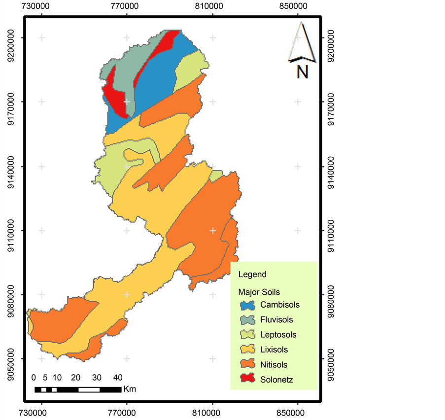
Figure 2.Maps of the Little Ruaha watershed showing (a) land use and (b) major soils.
database for different soil types and profiles with important soil properties which can be extracted. Figure 2(b) shows the soil map with six major soil types domi- nant in the study watershed; Cambisols, fluvisols, leptosols, lixisols, nitisols and so- lonetz based on the FAO Classification.
As SWAT requires information on soil properties such as soil texture, hydrologic soil group (HSG), bulk density, soil depth, and organic matter, soil profiles in the study watershed were obtained from literature and from the World Soil Information website (http://www.soilgrids.org/). This is a collection of updatable soil property and class maps of the world at 1 km spatial resolution produced using state-of-the-art model base [47] . ISRIC-World Soils Information contains a database for different soil types and profiles with important soil properties can be extracted.
Climate data were obtained from the Tanzania Meteorogical Agency (TMA) and the Rufiji Basin Water Board (RBWB). Rainfall data for three stations Iringa Met, Msembe Met and Mtera Meteorological Station with different length periods were available (Table 1). Quality check was conducted on the dataset by evaluating consistency and checking for missing data. The period for which all the stations had data was chosen and used as inputs for the model. Other stations with less data were used for filling missing data using regression equations [48] . A stochastic weather generator (WEXGEN) [32] is built-in the SWAT and uses it for filling-in missing climate data gaps. The weather generator model uses monthly statistics calculated from daily weather data to account for the missing data in the daily time series and/or simulate weather based on the statistics [27] . Therefore, 12 years of data were used for calculating the statistics at monthly time scale that were used for building the WXGEN.
The dataset had different record lengths, and based on the availability of data for other variables such as temperature and relative humidity, starting from 1979 was considered a good approach. Weather data for Mtera and Iringa Meteorological stations were used. Additional weather data were obtained from reanal- ysis data from the WATCH Forcing Data Methodology applied to ERA-Interim data Meteorological Forcing (WFDEI) dataset [49] . The WFDEI dataset was co- rrelated with observed data and a fair agreement was found. In the absence of long record of temperature, relative humidity, wind and solar radiation data, these records were used.
2.2.3. Model Set Up and Calibration Approach
Watershed delineation process which includes processing of DEM data for stream network and sub-watershed delineation was done using the ArcSWAT (ArcGIS interface of the SWAT model) model version 2012.10.18. The watershed delineation process resulted into 31 sub-watersheds which were further subdivided into 698 HRUs based on the unique combination of land use and soil type. Recommended thresholds of 10% for land cover and 5% for the soil area were applied to limit the number of HRUs in each watershed.
The curve number method was chosen for estimating rainfall-runoff in the watershed, while daily curve number was determined using the Plant ET method, potential evapotranspiration was estimated using the Hargreaves method and the variable storage was used for channel routing. The HRU management file is used to summarize land-use characteristics in SWAT. The file contains input data on planting, harvesting, irrigation applications, nutrient and pesticide applications as well as tillage applications. Three databases are used in SWAT to store information required for plant growth, urban land characteristics and

Table 1. Rain gauge stations in the little Ruaha Watershed used in this study.
fertilizer components. Three important land-use parameters are CNII value, CANMX (maximum canopy storage for each land use) and ALAI (initial leaf area index). The primary SWAT files used to summarize land-use characteristics is the HRU management file (.mgt).
Operation schedules for the four common crops (two cereals and two horticultural crops) available in the study area were included in the management file and were obtained from socio-economic surveys. The cereal crops are maize and rice and the two horticultural are tomato and onions. The horticultural crops were restricted in the lowlands and were therefore implemented in areas with a slope below or equal to 5%.
2.2.4. Sensitivity and Uncertainty Analysis
In order to understand how closely the model simulates the hydrological processes within a watershed, it is critical to examine the influence of different parameters. SWAT is a physically based process model that uses spatially-variable inputs such as land use, elevation, soil and other different hydrological parameters. Therefore, SWAT has many parameters, and due to the nature of the simulations and computational constrains, it is difficult to calibrate all the parameters. In order to understand the model performance, a sensitivity analysis for quantifying the most sensitive parameters is carried out prior to model calibration. This helps to ascertain whether the appropriate quantity and quality of data can be obtained to provide realistic model outputs given parameter sensitivity. In this study, a sensitivity analysis using the Sequential Uncertainty Fitting (SUFI-2) within the SWAT-CUP model [50] was used. Initial run of the SWAT- CUP was set using as many parameters as 23 that are responsible for surface runoff, groundwater and other hydrological processes within the watershed. The advantage of using SWAT-CUP lies on the possibility of using different kinds of parameters including those responsible for surface runoff, water quality parame- ters, crop, parameters, crop rotation and management parameters, and weather generator parameters.
2.2.5. Model Calibration and Evaluation
Calibration in this study was carried out in order to improve model performance using data from outlets in three sub-basins which are located in the upstream, middle and downstream areas. As the model was set using the baseline land use, the data for calibration was divided to coincide with that period. However, due to dearth of flow data in the study area, calibration was done from 1989 to 1998 following a warm-up period which was intended to allow the model parameters reach a steady-state condition. Evaluation period was a seven years period from 1999 to 2005. The flow gauging stations used are shown in Table 2. Calibration was done for daily and monthly simulations. The calibration and evaluation processes were carried out using the Sequential Uncertainty Fitting (SUFI-2) in the semi-automatic SWAT-CUP model [50] which was developed to include methods by Van Griensven and Bauwens [51] and other approaches.
SUFI-2 uses a semi-automated approach that incorporates both manual and
Table 2. Streamflow gauge stations in the little Ruaha River watershed used in this study.
auto-calibration procedures including the sensitivity and uncertainty analysis [41] . This allows users to adjust manually some parameters and range iteratively between auto-calibration runs. In SUFI-2, parameter uncertainty accounts for all sources of uncertainties such as uncertainty in driving variables [50] . Quantification of the uncertainties is done using the P-factor, which is the percentage of measured data bracketed by the 95% prediction uncertainty (95 PPU). The 95PPU is calculated at the 2.5% and 97.5% levels of cumulative distribution of an output variable obtained through Latin hypercube sampling, disallowing 5% of the worst simulations. Another measure quantifying the strength of a calibration/uncertainty analysis is the d-factor, which is the average thickness of the 95PPU band divided by the standard deviation of the measured data. Thus SUFI-2 seeks to bracket most of the measured data with the smallest possible uncertainty band [50] . SUFI-2 has been successfully used for case studies in different parts of the world [41] [52] [53] . Parameters that are responsible for surface flow and groundwater were used in the calibration process. The calibration process involved adjusting the model’s input parameters as guided by the sensitivity analysis, to match the observed and simulated streamflows. In order to have an idea on the influence of groundwater on the flow in the three basins used for calibration, hydrograph separation was implemented using the Web GIS-based Hydrograph Analysis Tool (WHAT) [54] using the recursive digital filter method for baseflow separation. The approach has been in other areas with similar land uses [55] [56] .
2.2.6. Model Performance
Model performance was carried out in order to verify the robustness of the model to simulate hydrological processes. The model performance in this study was carried out based on [57] model evaluation guideline. Therefore, the Nash- Sutcliffe Efficiency (NSE) [58] , percent bias (PBIAS) and ratio of the root mean square to the standard deviation of measured data (RSR) were used. The NSE indicates how well the plot of observed versus simulated value fits the 1:1 line and is computed as the ratio of residual variance to measured data variances [58] . NSE values range between  and 1 (inclusive), if NSE is less than or close to zero, the model prediction is considered unacceptable and means that the model prediction is no better than using average annual runoff volume as predictor of runoff. If the values approach one, the model predictions are considered to be acceptable. Results between zero and 1 are indicative of the most efficient parameters for model predictive ability, and NSE values of 1 indicate perfect alignment between simulated and observed values. This method has been commonly used in judging model performance in many hydrological modeling studies (e.g. [27] [53] [57] ), which provides extensive information on reported values.
The NSE is calculated by:
 (1)
(1)
where NSE is the Nash-Sutcliffe Efficiency, Qmeas is the measured flow, Qsim is the simulated flow and  is the mean of measured flow at the outlet.
The Percent bias (PBIAS) measures the average tendency of the simulated data to be larger or smaller than their observed counterparts [59] . The PBIAS is calculated as:
 (2)
(2)
where Qmeas is the measured flow and Qsim is the simulated flow. The optimal value of PBIAS is 0.0, with low-magnitude values indicating accurate model simulation. Positive values indicate model underestimation bias, and negative values indicate model overestimation bias [59] .
The ratio of root mean square error to the standard deviation of measured data (RSR) is calculated as the ratio of the Root Mean Square Error (RMSE) and standard deviation of the observed data.
 (3)
(3)
Model simulation is judged as satisfactory if NSE > 0.5, RSR ≤ 0.70 and PBIAS ±25% [53] [57] .
3. Results and Discussion
3.1. Sensitivity Analysis
Table 3 shows the list of 10 parameters that were the most sensitive for flow prediction in the model. The ranking shown is from the most sensitive with 1 being the most sensitive. It was found that the curve number (CN2) was the most sensitive parameter, followed by the base flow alpha factor (ALPHA-BF), groundwater delay time (GW_DELAY), threshold water depth in the shallow aquifer (GWQMN), and groundwater “revap” coefficient (GW-REVAP).
The most significant parameters were considered for further model calibration. The rest of the parameters had no significant effect on streamflow simulations; altering values would not yield any significant changes in the model output.
Table 3. Ranking of the 10 most sensitive parameters in the Little Ruaha River Watershed (from the most sensitive) and their fitted value parameters.
3.2. Calibration and Evaluation of Results
As described earlier, calibration was done in three sub-basins located in the upstream (Reach No.27), middle (Reach No.19) and downstream (Reach No.7) for 1KA32A Little Ruaha River at Makalala, 1KA21A Little Ruaha River at Ihimbu and 1KA31 Little Ruaha River at Mawande respectively. The best fitted parameter values for the calibration process are as shown in Table 3. Table 4 shows the results of calibrated and evaluation values at the monthly time step. Table 4 shows the calibrated and evaluation values and Figure 3 and Figure 4 show hydrograph comparison between the measured and simulated streamflows at 1KA31 and 1KA32A during calibration and evaluation. Comparison of the results between the measured and calibrated streamflows show a good agreement with NSE, PBIAS and RSR statistical values falling within the range of good to very good models. NSE values for monthly streamflow calibration and evaluation ranged from 0.64 to 0.77. According to the model evaluation guidelines, SWAT 2012 simulated the streamflow fairly well, as shown by statistical results, and supported by the graphical results in Figure 3. The PBIAS values ranged from −12.3% to 1.8% during calibration and from −28.3% to 10.2% during evaluation. The RSR values varied from 0.48 to 0.60 during both calibration and evaluation. These values indicate that the model performance for streamflow residual variation ranged from good to very good. In general, from the results shown in Table 4, the simulated results from the model show good results during calibration and evaluation processes for the three sub-basins. The simulated mean monthly streamflow at 1KA31 (sub-basin) was 17.92 m3/s while the observed was 21.58 m3/s at monthly time step. It was also observed that the mean streamflow at gauging station 1KA21A (Sub-Basin 19) was 11.31 m3/s for the observed and 8.81 m3/s for the simulated. The difference was not significant for the third gauging station, where the observed monthly streamflow was 3.08 m3/s compared with the simulated 2.93 m3/s.
Table 4. Results of streamflow model output for the calibration and evaluation processes based on the developed model evaluation guidelines at monthly time step.
![]()
![]()
Figure 3. Comparison of observed and simulated streamflows at two gauging stations in the Little Ruaha Watershed for the calibration stage.
Daily calibration was conducted for the data from two sub-basins (Little Ruaha at Mawande and Little Ruaha at Makalala) for the period of 7 years from 1999 to 2005. Due to lengthy periods of data gaps, gauging station 1KA21A Little Ruaha at Ihimbu was not included in the evaluation process at daily time steps. Results of the calibration and evaluation are shown in Table 5. Results further
![]()
![]()
Figure 4. Comparison of observed and simulated streamflows at two gauging stations in the Little Ruaha Watershed for the evaluation stage.
Table 5. Results of streamflow model output for the calibration and evaluation processes based on the developed model evaluation guidelines at daily time step.
show the simulated mean daily streamflow was 17.52 m3・s−1 and observed mean daily flow was 23.06 m3・s−1 for gauging station 1KA31 and for gauging station 1KA32A, the simulated mean streamflow was 2.89 m3・s−1 while the observed mean daily stream flow was 3.21 m3・s−1.
Based on the statistical and graphical evaluation, the model was considered reasonable and could be used for analyses of hydrological processes within the watershed including water balance, land use and land cover impacts and other issues. Moriasi, Arnold [57] proposed that in order for a model to be judged as satisfactory for hydrological and pollutant loss evaluations it should at least have NSE values of 0.5 or more [41] at monthly time steps. Despite data challenges for the study watershed, the model results were deemed reasonable. Other studies in the region have reported different calibration and evaluation results depending on data quality. For example, Birhanu [30] reported NSE values ranging between 11% and 63.3% in the Kihansi River catchment, Natkhin, Dietrich [31] reported R2 values of between 13% and 57% for Morogoro and Mgude watersheds.
3.3. Implications and Application of Results for Further Hydrological Analysis
Long term simulation results for the period between 1990 to 2012 for 1KA31A (Little Ruaha at Mawande) which happens to be located in the downstream area show reasonable model prediction of streamflow with the average annual streamflow of 22.87 m3・s−1 in comparison to the observed average annual flow of 21.01 m3・s−1. The results show good agreement between the observed and predicted streamflows at the downstream outlet (1KA31A). This is confirmed by long term monthly simulation shown in Figure 5. The hydrographs show good agreement between the observed and the simulated streamflows with R2 = 0.81. As it can be observed from Figure 5 that simulated had a tendency of over-pre- dicting peak flows and under-predicting baseflow in some situations, but the general pattern seemed to be within the range of the observed streamflow.
3.3.1. Infilling Missing Data and Generation of Complete Discharge Time Series
The calibrated and validated SWAT model was used to simulate the daily flow time series at the three sub-basins namely Little Ruaha River at Makalala, Ihimbu and Mawande. Missing data is a challenge in Tanzania [31] [60] and is a major source of uncertainty in hydrological analyses. Data gaps in most rivers in Tanzania occurred from the early 1980s [61] and Little Ruaha River was not an exception. Figure 6 presents the time series of average daily streamflow after gap
![]()
Figure 5. Observed and predicted hydrographs of streamflow (m3/s) at 1KA31A (Little Ruaha at Mawande) 1990-2012.
![]()
Figure 6. Time series of average daily streamflow (m3/s) for Little Ruaha River at Makalala (a) and at Mawande (b).
filling. The dataset is the most complete time series to be available for the watershed. Data filling using SWAT was judged to be more robust for predicting low flows compared to Artificial Neural Network in a study by [62] , and is more favored than statistical approaches because the latter assumes the datasets are linear and stationery.
3.3.2. Average Annual Flow
Figure 7 presents the average annual flows fitted with linear trend lines for the Little Ruaha River at Makalala and Mawande. The trend lines have negative slopes indicating the decline in magnitude of annual flows over time. Nevertheless, the nature of the slope is not uniform at all the stations. The slope of trend line at Makalala station is steeper as compared to Mawande stations. The average annual flow volume is 127.4 Mm3 at Makalala and 741.5 Mm3 at Mawande.
3.3.3. River Flow Trends
Seasonal and inter-annual variability
To statistically assess if there is a monotonic upward or downward trend in seasonal and inter-annual flows over time, a Mann-Kendall (MK) test was performed [63] [64] . A monotonic upward (downward) trend means that the variable
![]()
![]()
Figure 7. Average annual (HY) flow (m3/s) for Little Ruaha River at two gauging stations fitted with a linear trend line.
consistently increases through time, but the trend may or may not be linear. The MK test can be used in place of a parametric linear regression analysis, which can be used to test if the slope of the estimated linear regression line is different from zero. It is important noting that the other regression analysis requires that the residuals from the fitted regression line be normally distributed; an assumption not required by the MK test, that is, the MK test is a non-parametric (distribution-free) test. Thus, Table 6 presents the results of trend analyses on annual and seasonal flows Little Ruaha River at Makalala, Ihimbu and Mawande gauging stations. The Mann-Kendall test statistics (Z) on annual and seasonal flows indicate decreasing trend in river flows in the catchment. The results suggest that the flows in the Little Ruaha Catchment are changing with time.
3.3.4. Flow Duration Curves
The shape of flow duration curves (FDCs) are related to the interactions of climate, catchment size and morphology, vegetation cover, and the properties of the subsurface domain, which together control the various runoff components [65] . The shape of FDCs is largely governed by both precipitation and evapotranspiration variability and how water moves through the catchment [65] . The
Table 6. Mann-Kendall test statistic (Z) results in seasonal mean and annual flows for Little Ruaha River at Makalala, Ihimbu and Mawande gauging stations.
Note: ***if trend at α = 0.001 level of significance, **if trend at α = 0.01 level of significance; *if trend at α = 0.05 level of significance, if cell is blank, the significance level is greater than 0.1.
FDC can be partitioned into three distinct parts [66] , each of which is governed by different mechanisms or process controls:
1) The upper part, which represent high flows, is governed by flood processes for which the dominant control is the interaction of extreme rainfall and fast runoff processes;
2) The middle part, relates to the mean runoff and its seasonality, for which the dominant control is the competition and seasonal interaction between available water, energy and storage, and
3) The lower part is governed by base flow recession behaviour over dry periods for which the dominant control is the competition between deep drainage and riparian zone evaporation.
In this study the FDC percentage points were calculated from the average daily flows data after filling gaps in the time series. The daily flow duration curves at Makalala, Ihimbu and Mawande are presented in Figure 8. The general outlook reveals steep slope for high flows (say at <Q5) indicating flushing catchment. Such phenomena could be attributable to change in land use and land cover. The results further indicate that for flow less that Q95 the river is almost at bed level. This means that water abstractions must be regulated to ensure the ecological integrity of the river. An environmental flow assessment will provide more guides on how to address this requirement.
![]()
Figure 8. 1-Day flow duration curve for Little Ruaha River at Makalala, Ihimbu and Mawande.
4. Discussion
The calibration of the model at monthly time steps at the outlet of the three subs-watersheds showed that the model deviated from the observed data by 7%, 9% and 1% for Mawande, Ihimbu and Makalala outlets, respectively. While the average simulated streamflow showed a slight over-prediction for Mawande and Ihimbu, the results showed model under-prediction for Makalala outlet. Results for the evaluation stage showed that the discrepancy between the simulated and observed streamflow was 22% for Mawande, 11% for Ihimbu and 22.2% for Makalala. It can be realized that the overall accuracy was lower during the evaluation period compared to the calibration period. Despite the slight discrepancies, visual inspection of hydrographs show that the simulated streamflows were within the range of the measured streamflows. Overall assessment of the model at both daily and monthly time steps showed a satisfactory results for baseflow and peak flows. Challenges of data for modeling and hydrological analysis in Tanzania have been highlighted by other researchers [28] [29] [30] [31] . By comparing the mean of the observed streamflow data from 1980 to 2012 before and after filling missing gaps, we found a deviation of 3%, signifying that the gap filling did not change the pattern of the data. SWAT has been used successfully by other researchers for gap filling of missing data and is considered one of the robust methods [62] . In a watershed that is faced with diverse and increased anthropogenic activities and competing demands for water, a complete set of streamflow data is important for sustainable water management. Studies such as environmental flow, water allocation and water availability as risks and disaster assessment are highly dependent on availability of good datasets.
5. Conclusions
The hydrology of the Little Ruaha River has been studied. Analysis of available historical river flow records revealed presence of many data gaps that necessitated conducting rainfall-runoff modelling using a Soil and Water Assessment Tool (SWAT). The model has been calibrated, verified and found to be adequate in simulating flows with high confidence. The model has been applied to simulate flows that were used in gap filling the missing data and thus generating complete daily time series of discharges at the three gauging stations of Makalala, Ihimbu and Mawande.
Further analysis on daily time series enabled computation of trends, flow duration curves, monthly and annual flows. The trend analysis on seasonal and annual flows revealed declining flows indicating that the flows are significantly changing with time. The decline in river flows will have some implications on the planned future water development in the catchment. There is therefore, a need to carry out analysis on the implications of water allocations (water use permits) on river flows. Along, this will be a need to understand the implications of water allocations on environmental flows for meeting the ecosystem ecological requirements.
The water balance of the Little Ruaha River catchment has not been fully evaluated including the impacts of planned interventions associated with land use/land cover changes. This will be part of the next phase of the study by applying a calibrated and verified SWAT model in understanding the future impacts of land use/land cover change on hydrological processes within the watershed including the water balance.
Acknowledgements
The authors highly acknowledge the financial support from the CGIAR Research Program on Water, Land and Ecosystems in the Nile and East Africa Region (WLE Nile-East Africa). WLE Nile-East Africa is a research-for-development initiative that seeks to restore and bolster opportunities for increased agricultural productivity through key ecosystem services, especially in the resource poor areas of the region. The CGIAR Research Program on Water, Land and Ecosystems (WLE) is a global research program that promotes a new approach to sustainable agricultural intensification in which a healthy functioning ecosystem is seen as a prerequisite to agricultural development, resilience of food systems and human well-being. This program is led by the International Water Management Institute (IWMI), a member of the CGIAR Consortium, and is supported by CGIAR, a global research partnership for a food-secure future. The authors also thank the valuable inputs received from the three anonymous reviewers. Our appreciation also goes to the Rufiji Basin Water Office and all the people consulted during the research.
Cite this paper
Mbungu, W.B. and Kashaigili, J.J. (2017) Assessing the Hydro- logy of a Data-Scarce Tropical Watershed Using the Soil and Water Assessment Tool: Case of the Little Ruaha River Watershed in Iringa, Tanzania. Open Journal of Modern Hydrology, 7, 65-89. https://doi.org/10.4236/ojmh.2017.72004
References
- 1. Carpenter, S.R. and Biggs, R. (2009) Freshwaters: Managing across Scales in Space and Time, in Principles of Ecosystem Stewardship. Springer, New York, 197-220.
https://doi.org/10.1007/978-0-387-73033-2_9 - 2. MEA (2005) Millenium Ecosystems Assessment: Ecosystems and Human Well-Being. Vol. 5, Island Press, Washington DC.
- 3. Dudgeon, D., et al. (2006) Freshwater Biodiversity: Importance, Threats, Status and Conservation Challenges. Biological Reviews, 81, 163-182.
https://doi.org/10.1017/S1464793105006950 - 4. WLE (2014) Ecosystem Services and Resilience Framework. CGIAR Research Program on Water, Land and Ecosystems (WLE). International Water Management Institute (IWMI), Colombo, 46p.
https://doi.org/10.5337/2014.229 - 5. FAO (Food and Agriculture Organization of the United Nations) (2011) FAOSTAT Database.
http://faostat3.fao.org/download/E/EL/E - 6. Foley, J.A., DeFries, R., Asner, G.P., Barford, C., Bonan, G., Carpenter, S.R., Helkowski, J.H., et al. (2005) Global Consequences of Land Use. Science, 309, 570-574.
https://doi.org/10.1126/science.1111772 - 7. Foley, J.A., Ramankutty, N., Brauman, K.A., Cassidy, E.S., Gerber, J.S., Johnston, M., Balzer, C., et al. (2011) Solutions for a Cultivated Planet. Nature, 478, 337-342.
https://doi.org/10.1038/nature10452 - 8. World Bank (2014) World Development Indicators: Agricultural Inputs.
http://wdi.worldbank.org/table/3.2 - 9. Tumbo, S.D., Kahimba, F.C., Mbilinyi, B.P., Rwehumbiza, F.B., Mahoo, H.F., Mbungu, W.B. and Enfors, E. (2012) Impact of Projected Climate Change on Agricultural Production in Semi-Arid Areas of Tanzania: A Case of Same District. African Crop Science Journal, 20, 453-463.
- 10. URT, Ministry of Agriculture, Food Security and Cooperatives (MAFC) (2015) Tanzania Agriculture Climate Resilience Plan, 2014-2019. Report 83, Ministry of Agriculture, Food Security and Cooperatives (MAFC), Dar Es Salaam.
http://www.agriculture.go.tz/publications - 11. Fischer, G., Shah, M., Tubiello, F.N. and Van Velhuizen, H. (2005) Socio-Economic and Climate Change Impacts on Agriculture: An Integrated Assessment, 1990-2080. Philosophical Transactions of the Royal Society B: Biological Sciences, 360, 2067-2083.
https://doi.org/10.1098/rstb.2005.1744 - 12. Cassman, K.G., Dobermann, A., Walters, D.T. and Yang, H. (2003) Meeting Cereal Demand While Protecting Natural Resources and Improving Environmental Quality. Annual Review of Environment and Resources, 28, 315-358.
https://doi.org/10.1146/annurev.energy.28.040202.122858 - 13. URT (2012) Tanzania National Climate Change Strategy. Division of Environment, Vice President’s Office, 92.
- 14. Mbungu, W. (2015) Climate Change Vulnerability Assessment in the Lake Rukwa Basin. Lake Rukwa Basin Water Board, Mbeya, 61.
- 15. Mbungu, W.B. (2016) Impacts of Land Use and Land Cover Changes, and Climate Variability on Hydrology and Soil Erosion in the Upper Ruvu Watershed, Tanzania. PhD Dissertation at Virginia Tech, Blacksburg.
- 16. Mbungu, W.B., Mahoo, H.F., Tumbo, S.D., Kahimba, F.C., Rwehumbiza, F.B. and Mbilinyi, B.P. (2015) Using Climate and Crop Simulation Models for Assessing Climate Change Impacts on Agronomic Practices and Productivity, in Sustainable Intensification to Advance Food Security and Enhance Climate Resilience in Africa. Springer, New York, 201-219.
https://doi.org/10.1007/978-3-319-09360-4_10 - 17. Mourice, S.K., Mbungu, W. and Tumbo, S.D. (2017) Quantification of Climate Change and Variability Impacts on Maize Production at Farm Level in the Wami River Sub-Basin, Tanzania, in Quantification of Climate Variability, Adaptation and Mitigation for Agricultural Sustainability. Springer, New York, 323-351.
https://doi.org/10.1007/978-3-319-32059-5_13 - 18. Elisa, M., Gara, J.I. and Wolanski, E. (2010) A Review of the Water Crisis in Tanzania’s Protected Areas, with Emphasis on the Katuma River—Lake Rukwa Ecosystem. Ecohydrology & Hydrobiology, 10, 153-165.
- 19. Kajembe, G.C., Mbwilo, A.J., Kidunda, R.S. and Nduwamungu, J. (2003) Resource Use Conflicts in Usangu Plains, Mbarali District, Tanzania. The International Journal of Sustainable Development & World Ecology, 10, 333-343.
https://doi.org/10.1080/13504500309470109 - 20. Nindi, S.J., Maliti, H., Bakari, S., Kija, H. and Machoke, M. (2014) Conflicts over Land and Water Resources in the Kilombero Valley Floodplain, Tanzania.
- 21. Mtahiko, M.G.G., Gereta, E., Kajuni, A.R., Chiombola, E.A.T., Ng’umbi, G.Z., Coppolillo, P. and Wolanski, E. (2006) Towards an Ecohydrology-Based Restoration of the Usangu Wetlands and the Great Ruaha River, Tanzania. Wetlands Ecology and Management, 14, 489-503.
https://doi.org/10.1007/s11273-006-9002-x - 22. SAGCOT (Southern Agricultural Growth Corridor of Tanzania) (2011) Southern Agricultural Growth Corridor of Tanzania Investment Blueprint. Dar Es Salaam.
- 23. Kadigi, R.M., Mdoe, N.S., Lankford, B.A. and Morardet, S. (2005) The Value of Water for Irrigated Paddy and Hydropower Generation in the Great Ruaha, Tanzania. Proceedings of the East Africa Integrated River Basin Management Conference, Morogoro, 7-9 March 2005, 265-278.
- 24. Kashaigili, J.J., Kadigi, R.M., Lankford, B.A., Mahoo, H.F. and Mashauri, D.A. (2005) Environmental Flows Allocation in River Basins: Exploring Allocation Challenges and Options in the Great Ruaha River Catchment in Tanzania. Physics and Chemistry of the Earth, Parts A/B/C, 30, 689-697.
- 25. Kashaigili, J.J, Kadigi R.M.J.,Mbungu, W.B., Sikira, A., Sirima, A., Placid, J.K., Mbwambo, E. and Minde, A. (2016) Laying the Foundations for Effective Landscape-Level Planning for Sustainable Development in the SAGCOT Corridor: Ihemi Agricultural Development Cluster (LiFELand). Draft Report Submitted to TNC, Sokoine University of Agriculture, Morogoro, 153 p.
- 26. Arnold, J.G., et al. (1998) Large Area Hydrologic Modeling and Assessment Part I: Model Development 1. Wiley Online Library, Hoboken.
- 27. Baker, T.J. and Miller, S.N. (2013) Using the Soil and Water Assessment Tool (SWAT) to Assess Land Use Impact on Water Resources in an East African Watershed. Journal of Hydrology, 486, 100-111.
https://doi.org/10.1016/j.jhydrol.2013.01.041 - 28. Mulungu, D.M. and Munishi, S.E. (2007) Simiyu River Catchment Parameterization Using SWAT Model. Physics and Chemistry of the Earth, Parts A/B/C, 32, 1032-1103.
https://doi.org/10.1016/j.pce.2007.07.053 - 29. Ndomba, P., Mtalo, F. and Killingtveit, A. (2008) SWAT Model Application in a Data Scarce Tropical Complex Catchment in Tanzania. Physics and Chemistry of the Earth, Parts A/B/C, 33, 626-632.
https://doi.org/10.1016/j.pce.2008.06.013 - 30. Birhanu, B.Z. (2009) Hydrological Modeling of the Kihansi River Catchment in South Central Tanzania Using SWAT Model. International Journal of Water Resources and Environmental Engineering, 1, 1-10.
- 31. Natkhin, M., Dietrich, O., Schafer, M.P. and Lischeid, G. (2015) The Effects of Climate and Changing Land Use on the Discharge Regime of a Small Catchment in Tanzania. Regional Environmental Change, 15, 1269-1280.
https://doi.org/10.1007/s10113-013-0462-2 - 32. Neitsch, S.L., Arnold, J.G., Kiniry, J.R., Williams, J.R. and King, K.W. (2002) Soil and Water Assessment Tool Theoretical Documentation. USDA-ARS Publication GSWRL 02-01 BRC 02-05 TR-01, USDA-ARS Publication, Washington DC.
- 33. Arnold, J.G. and Fohrer, N. (2005) SWAT2000: Current Capabilities and Research Opportunities in Applied Watershed Modelling. Hydrological Processes, 19, 563-572.
https://doi.org/10.1002/hyp.5611 - 34. Arnold, J. and Allen, P. (1996) Estimating Hydrologic Budgets for Three Illinois Watersheds. Journal of Hydrology, 176, 57-77.
https://doi.org/10.1016/0022-1694(95)02782-3 - 35. Dessu, S.B. and Melesse, A.M. (2012) Modelling the Rainfall-Runoff Process of the Mara River Basin Using the Soil and Water Assessment Tool. Hydrological Processes, 26, 4038-4049.
https://doi.org/10.1002/hyp.9205 - 36. Perrin, J., Ferrant, S., Massuel, S., Dewandel, B., Maréchal, J.C., Aulong, S. and Ahmed, S. (2012) Assessing Water Availability in a Semi-Arid Watershed of Southern India Using a Semi-Distributed Model. Journal of Hydrology, 460-461, 143-155.
https://doi.org/10.1016/j.jhydrol.2012.07.002 - 37. Asres, M.T. and Awulachew, S.B. (2010) SWAT Based Runoff and Sediment Yield Modelling: A Case Study of the Gumera Watershed in the Blue Nile Basin. Ecohydrology & Hydrobiology, 10, 191-199.
- 38. White, E.D., Easton, Z.M., Fuka, D.R., Collick, A.S., Adgo, E., McCartney, M., Steenhuis, T.S., et al. (2011) Development and Application of a Physically Based Landscape Water Balance in the SWAT Model. Hydrological Processes, 25, 915-925.
https://doi.org/10.1002/hyp.7876 - 39. Jha, M., Pan, Z., Takle, E.S. and Gu, R. (2004) Impacts of Climate Change on Streamflow in the Upper Mississippi River Basin: A Regional Climate Model Perspective. Journal of Geophysical Research: Atmospheres, 109.
https://doi.org/10.1029/2003JD003686 - 40. Neitsch, S.L., Williams, J.R., Arnold, J.G. and Kiniry, J.R. (2011) Soil and Water Assessment Tool Theoretical Documentation Version 2009. Texas Water Resources Institute, College Station.
- 41. Arnold, J.G., Moriasi, D.N., Gassman, P.W., Abbaspour, K.C., White, M.J., Srinivasan, R., Kannan, N., et al. (2012) SWAT: Model Use, Calibration, and Validation. Transactions of the ASABE, 55, 1491-1508.
https://doi.org/10.13031/2013.42256 - 42. Gassman, P.W., Reyes, M.R., Green, C.H. and Arnold, J.G. (2007) The Soil and Water Assessment Tool: Historical Development, Applications, and Future Research Directions. Transactions of the ASABE, 50, 1211-1250.
https://doi.org/10.13031/2013.23637 - 43. Breiman, L. (2001) Random Forests. Machine Learning, 45, 5-32.
https://doi.org/10.1023/A:1010933404324 - 44. Rodriguez-Galiano, V.F., Ghimire, B., Rogan, J., Chica-Olmo, M. and Rigol-Sanchez, J.P. (2012) An Assessment of the Effectiveness of a Random Forest Classifier for Land-Cover Classification. ISPRS Journal of Photogrammetry and Remote Sensing, 67, 93-104.
https://doi.org/10.1016/j.isprsjprs.2011.11.002 - 45. De Pauw, E. (1984) Soils, Physiography and Agroecological Zones of Tanzania. Ministry of Agriculture, Dar-es-Salaam, Tanzania/FAO, Rome.
- 46. Batjes, N.H. (2004) SOTER-Based Soil Parameter Estimates for Southern Africa. ISRIC-World Soil Information, Wageningen DC.
- 47. ISRIC (2013) ISRIC—World Soil Information.
http://www.soilgrids.org/ - 48. McCuen, R.H. (2003) Modeling Hydrologic Change: Statistical Methods. Lewis Publishers, Boca Raton, 433 p.
- 49. Weedon, G.P., Balsamo, G., Bellouin, N., Gomes, S., Best, M.J. and Viterbo, P. (2014) The WFDEI Meteorological Forcing Data Set: WATCH Forcing Data Methodology Applied to ERA—Interim Reanalysis Data. Water Resources Research, 50, 7505-7514.
https://doi.org/10.1002/2014WR015638 - 50. Abbaspour, K., Vejdani, M. and Haghighat, S. (2007) SWAT-CUP Calibration and Uncertainty Programs for SWAT. MODSIM 2007 International Congress on Modelling and Simulation, December 2007, 1596-1602.
- 51. Van Griensven, A. and Bauwens, W. (2003) Multiobjective Autocalibration for Semidistributed Water Quality Models. Water Resources Research, 39.
https://doi.org/10.1029/2003wr002284 - 52. Abbaspour, K.C., et al. (2009) Assessing the Impact of Climate Change on Water Resources in Iran. Water Resources Research, 45.
https://doi.org/10.1029/2008WR007615 - 53. Betrie, G.D., Mohamed, Y.A., Griensven, A.V. and Srinivasan, R. (2011) Sediment Management Modelling in the Blue Nile Basin Using SWAT Model. Hydrology and Earth System Sciences, 15, 807-818.
https://doi.org/10.5194/hess-15-807-2011 - 54. Lim, K.J., Park, Y.S., Kim, J., Shin, Y.C., Kim, N.W., Kim, S.J., Engel, B.A., et al. (2010) Development of Genetic Algorithm-Based Optimization Module in WHAT System for Hydrograph Analysis and Model Application. Computers & Geosciences, 36, 936-944.
https://doi.org/10.1016/j.cageo.2010.01.004 - 55. Recha, J.W., Lehmann, J., Walter, M.T., Pell, A., Verchot, L. and Johnson, M. (2012) Stream Discharge in Tropical Headwater Catchments as a Result of Forest Clearing and Soil Degradation. Earth Interactions, 16, 1-18.
https://doi.org/10.1175/2012EI000439.1 - 56. Longobardi, A. and Villani, P. (2008) Baseflow Index Regionalization Analysis in a Mediterranean Area and Data Scarcity Context: Role of the Catchment Permeability Index. Journal of Hydrology, 355, 63-75.
https://doi.org/10.1016/j.jhydrol.2008.03.011 - 57. Moriasi, D.N., Arnold, J.G., Van Liew, M.W., Bingner, R.L., Harmel, R.D. and Veith, T.L. (2007) Model Evaluation Guidelines for Systematic Quantification of Accuracy in Watershed Simulations. Transactions of the ASABE, 50, 885-900.
https://doi.org/10.13031/2013.23153 - 58. Nash, J.E. and Sutcliffe, J.V. (1970) River Flow Forecasting through Conceptual Models Part I—A Discussion of Principles. Journal of Hydrology, 10, 282-290.
https://doi.org/10.1016/0022-1694(70)90255-6 - 59. Gupta, H.V., Sorooshian, S. and Yapo, P.O. (1999) Status of Automatic Calibration for Hydrologic Models: Comparison with Multilevel Expert Calibration. Journal of Hydrologic Engineering, 4, 135-143.
https://doi.org/10.1061/(ASCE)1084-0699(1999)4:2(135) - 60. Mbungu, W., Ntegeka, V., Kahimba, F.C., Taye, M. and Willems, P. (2012) Temporal and Spatial Variations in Hydro-Climatic Extremes in the Lake Victoria Basin. Physics and Chemistry of the Earth, Parts A/B/C, 50, 24-33.
https://doi.org/10.1016/j.pce.2012.09.002 - 61. Ndomba, P.M. (2014) Streamflow Data Needs for Water Resources Management and Monitoring Challenges: A Case Study of Wami River Subbasin in Tanzania, in Nile River Basin. Springer, New York, 23-49.
https://doi.org/10.1007/978-3-319-02720-3_3 - 62. Kim, M., Baek, S., Ligaray, M., Pyo, J., Park, M. and Cho, K.H. (2015) Comparative Studies of Different Imputation Methods for Recovering Streamflow Observation. Water, 7, 6847-6860.
https://doi.org/10.3390/w7126663 - 63. Mann, H.B. (1945) Non-Parametric Test against Trend. Econometrica, 13, 245-259.
https://doi.org/10.2307/1907187 - 64. Kendall, M.G. (1975) Rank Correlation Methods. Charles Griffin, London.
- 65. Castellarin, A., Camorani, G. and Brath, A. (2007) Predicting Annual and Long-Term Flow-Duration Curves in Ungauged Basins. Advances in Water Resources, 30, 937-953.
https://doi.org/10.1016/j.advwatres.2006.08.006 - 66. Yokoo, Y. and Sivapalan, M. (2011) Towards Reconstruction of the Flow Duration Curve: Development of a Conceptual Framework with a Physical Basis. Hydrology and Earth System Sciences, 15, 2805-2819.
https://doi.org/10.5194/hess-15-2805-2011