Open Journal of Acoustics
Vol.3 No.1(2013), Article ID:29315,6 pages DOI:10.4236/oja.2013.31001
Calculation of Sound Ray’s Trajectories by the Method of Analogy to Mechanics at Ocean
Institute of Applied Physics, Russian Academy of Sciences, Nizhny Novgorod, Russia
Email: ivg@hydro.appl.sci-nnov.ru
Received September 10, 2012; revised October 14, 2012; accepted October 24, 2012
Keywords: Sound Rays; Material Particle; Analogy; Hamilton Equations
ABSTRACT
In this paper, one of analogies available in the literature between movement of a material particle and ray propagation of a sound in liquid is used. By means of the equations of Hamilton describing movement of a material particle, analytical expression of a tangent to a trajectory of a sound ray at non-uniform ocean on depth is received. The received expression for a tangent differs from traditional one, defined under law Snelius. Calculation of trajectories, and also other characteristics of a sound field is carried out by two methods: first—traditional, under law Snelius, and second—by the analogy to mechanics method. Calculations are made for canonical type of the sound channel. In the region near to horizontal rays, both methods yield close results, and in the region of steep slope, the small distinction is observed.
1. Introduction
The ray description of a sound field is widely applied in problems on sound propagation at ocean. It is because of the big accuracy with which the ray theory defines the basic characteristics of a sound field. Among modern computing means, the ray method of calculation of a sound field does not cause any difficulties. Advantage of this method consists that it contains a minimum quantity of approximations and can serve as the standard in an evaluation of other methods. It proves to be true, for example, when calculation of a sound field of caustics is made [1,2]. Unique restriction of use of a ray method is performance of conditions of geometrical acoustics in non-uniform spaces [3].
Along with a traditional ray method of calculation of a sound field at the ocean, using Snelius’s law, other methods based on analogy between propagation of a sound wave at ocean and movement of a material particle are widely applied, see for example [4]. Calculation of a trajectory of a material particle is made on the equations of classical mechanics and the equations of Hamilton. The analogy between movement of a sound wave and a material particle establishes connections between the functions describing their movement. In [4] and later works with a view of simplification, the following assumption is entered—the horizontal spatial co-ordinate of propagation of a sound wave is considered simultaneously and as time co-ordinate.
Other ways of an establishment of analogy between propagation of a sound and movement of a mechanical particle are offered in [3]. In this paper, all co-ordinates of a sound trajectory, time and spatial, keep the number and functional value at definition of a trajectory of a sound wave on the equations of Hamilton. It provides visibly demonstration and reliability of conformity of two various physical phenomena and possibility of their description by means of the same mathematical apparatus.
The purpose of the given work is to carry out one more variant of use of the equations of the classical mechanics, offered in [3], for calculation of a trajectory of propagation of a sound in a liquid. Analytical expression for a tangent to the ray trajectory, distinct from given by law Snelius is received. Comparison of calculation of trajectories and other characteristics of a sound field in a wave - guide by two methods, traditional under Snelius law and by analogy to classical mechanics, [3] is spent. The short description of this method of calculation of a trajectory by analogy to mechanics is resulted in [5].
It is known that in isotropic, homogeneous space not changing in time plane sound waves propagate in a direction of a wave vector k which does not vary neither on value, nor in a direction. At ocean, a sound speed depends on depth that makes the space not isotropic. It leads to the change of a wave vector k both on size, and in a direction. Therefore, the sound wave is not a plane one any more. However, representation about a plane wave can be used and in such space if on distances of an order of length of a wave, the value and a direction of a wave vector vary slightly. The method of replacement of a real sound wave with a set of plane waves is called as a method of geometrical acoustics [3]. In those cases where we will apply a method of geometrical acoustics, it is possible to enter concept about rays as about lines, tangents to which coincide with a direction of propagation of a plane wave on small regions of space. Thus, justice of a method of geometrical acoustics reduces a problem of propagation of a sound in the anisotropy space to calculation of ray trajectories.
2. Traditional Method Ray’s Calculation
Let’s consider briefly traditional way of definition of ray’s trajectories at ocean with speed of a sound depending on depth (a method 1). We will accept, that the ocean is a planelayered space in which speed of a sound varies with change depth z and does not depend on co-ordinates x, y. Thanks to uniform and isotropic space along axes x, y projections of a wave vector k on an axis  also do not depend on co-ordinates x, y, [3]. We will accept, that a plane of falling of a sound wave serves the plane x, z. Let θ—a corner between a vector direction k and an axis z. Then the running sound wave in a waveguide is described by following expression:
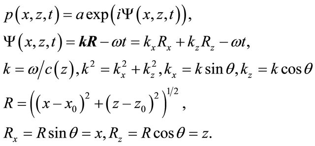 (1)
(1)
Here a—amplitude of a wave, —a wave phase (eikonal), k—a wave vector, k—its module (length), R—a vector of a trajectory of the wave, parallel to a vector k, R—the module (length) of a vector, co-ordinates of the beginning of vector R—x0, z0, end co-ordinates (current co-ordinates of a trajectory)—x, z. We will accept, that absorption of a sound is a little, the amplitude of a wave does not vary.
According to Snelius law the component of a wave vector 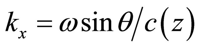 remains invariable for a concrete ray at non-uniform ocean on depth:
 (2)
(2)
Here z0—depth of a source of a sound, θ0—an angle of an departure of a ray from a source, —speed of a sound on depth of a source. According to Snelius law, Equation (2), if a refraction angle
  on depth
 , where
 , “const” in Equation (2) is equal to
 . Apparently from Equation (2), the constant
  can be expressed through an angle of departure of a ray from a source θ0 and speed of a sound
  too, “const”
 . We will accept, that on distances of several lengths of waves the module of a wave vector varies slightly, considerably its direction varies only. Therefore we will enter a single vector n1, coinciding on a direction with a wave vector,
 . Components of a single vector n1 are expressed through an angle
 . Using for a constant in Snelius law (2) expression
  we will receive:
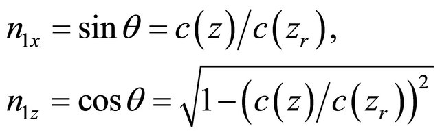 (3)
(3)
Equations (3) defines components of an single vector n1 along axes of co-ordinates, and also a tangent to a trajectory of propagation of a wave tgθ, coinciding on a direction with a vector k. From Equation (3) it is visible, that components n1x, n1z depend from z, n1x has the same dependence on depth, as . For a components of a wave vector taking into account Equation (3) we will receive:
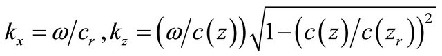 (4)
(4)
It is visible, that kx—a constant for the chosen ray with a turning point on depth zr, kz—depth function of z. Components of a wave vector, Equation (4), are received in the assumption, that periodicity of a sound field at change  is not broken, conditions of geometrical acoustics are applicable. Trajectory co-ordinates x, z and length of a trajectory l, are connected by known parities:
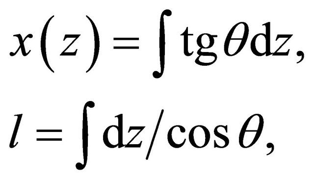 (5)
(5)
which allow to calculate with the big accuracy a trajectory, and also time of propagation of a sound along a trajectory. Convincing acknowledgement of accuracy of calculation of a sound trajectory by a ray method can be found in many works, for example, in [6] where the value of time of propagation of a sound on distance ~17000 km calculated under the ray theory and measured in experiment are resulted, coincided with each other. Thus, a method 1 of geometrical acoustics in partially isotropic space defines a tangent to a trajectory of a ray in the form of analytical function of speed of a sound on which the ray trajectory, time of propagation of a sound on a ray and the value of the sound field are calculated along a ray trajectory.
3. The Method of Analogy to Mechanics
Let’s consider another method, method 2, calculation of trajectories of the sound rays, based on analogy between movement of a material particle and sound propagation in approach of the geometrical acoustics, offered in [3].
Let us conceder briefly principal features of the classical mechanics, describing movement of a material particle by the equations of Hamilton [7]. Position of a material particle in the classical mechanics is defined by its generalized co-ordinates  and the generalized impulses
 , equal m
 , where m—mass and a
  projection of speed of a particle to an axis i, the index i means x, z. The generalized co-ordinate q in a homogeneous space is a particle radius-vector if the beginning of its movement coincides with the beginning of co-ordinates [7]. In this case projections of length of a vector q on an axis of co-ordinates coincide with values x, z, since
 . The same concerns and to a vector of the generalized speed. In the closed system where the particle is not exposed to any influence, a vector q is the straight line, and a vector p is a constant impulse of a particle, a constant value of speed. The big role in the classical mechanics plays the function of “action” S defined as integral along a trajectory, taken on time from Lagrange’s function between two points of a trajectory
  and
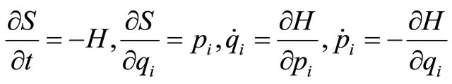
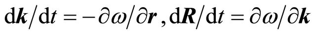
and  which the particle occupies during the set moments of time [7]. The derivative on time from action S defines Hamiltonian of material particle H, and on the generalized co-ordinate—a particle impulse. The equations of Hamilton can be received from a condition of existence of a minimum value of action S [7]. We bring these four equations which we use to establish correlation between movement of a material particle and propagation of a sound wave and for calculation of a sound trajectory:
 (6)
(6)
At known function of action S from first two equations it is defined Hamiltonian H of particle and its impulse p. From second two differential equations which are equations of Hamilton, co-ordinates of a trajectory of a particle qi and components of its speed  are calculated.
The equations of Hamilton define a particle trajectory, as well as Newton’s second equation. We will accept, that expression for eikonal  in the definition of the sound wave’s field, Equation (1), is analogue of action S of a material particle. One of the functions entering in Equation (1), is a trajectory of a sound wave (a ray on which the sound wave propagates), vector R. It is natural to accept, that vector R is analogue of a vector of the generalized co-ordinate q of the particle, and projections to axes of co-ordinates of a vector of trajectory Ri - analogue qi. Continuing analogy between S and Ψ we will receive from Equations (6) the first equation, that analogue Hamiltonian H is frequency of radiation,
  , and from the second equation—analogue of an impulse p of the particle is the wave vector k, pi - ki. It is already formal analogy between particle’s Hamiltonian H and frequency of a sound wave
  and components of the generalized vector pi and a wave vector ki. The equations of Hamilton, 3, 4 in Equation (6), for a trajectory of a sound wave look like:
 (7)
(7)
Let’s present a wave vector, as in a method 1, in the form of its module that don’t change on a distance of several wave’s lengths and single vector n2, that varies its direction,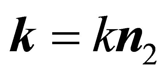 . We will receive from the Equations (7) at stationary propagation of a sound in the motionless non-uniform space the equations for vectors n2 and R:
 . (8)
. (8)
Authors [3] bring the equation for vector definition n2, containing an additional member, in our designations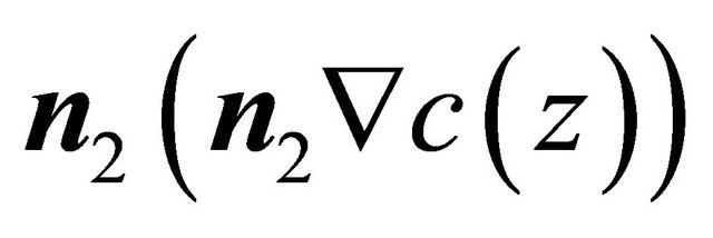 . This member has appeared at transition from
  to
to , through derivatives
 and replacement
  on
on
 , and
, and  on cn2
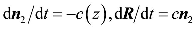
from Equation (8), the second one. It is incorrect procedure since the generalized functions q and p for a mechanical particle, together with their analogues R and k in a sound wave, depend by their primary definition only on variables x, z, t, but not from each other. Therefore the correct equation for vector’s definition n2 is the first in Equations (8). It is easy to show, that the decision of the equation for n2, resulted in [3] with an additional member , is the following:
 , i.e. is definition of an single wave vector, and its components values for a considered problem remain not defined.
Let’s write down system of the Equation (8) for projections of vectors R and n2 on an axis x, z:
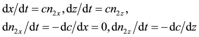 (8’)
(8’)
The decision of the third of Equation (8’) can be or  or
or . The first decision according to existing connection
  and
and  leads to
 . This decision is fair only in the isotropic spaces. Remains
 . Since the component of a single vector n2x can be expressed through
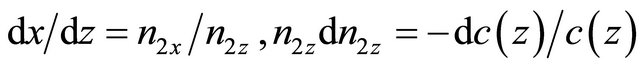
  becomes known after definition n2z. Using a method of the decision of system of the ordinary stationary differential equations of 1st order, [8], after exception differential dt from Equations (8’) we will receive two equations:
 (9)
(9)
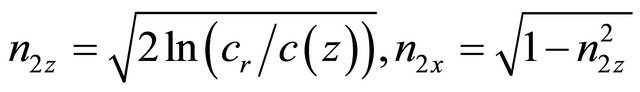
Solving the second of them, we will define a projection of a single vector n2z as function of depth 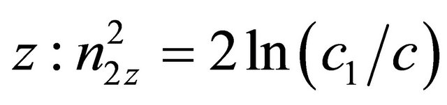 , where с1 – an integration constant. A constant с1 we will accept equal speed of a sound in a turning point of a ray, с1 = сr. As a result for n2x, n2z, we will receive following expressions:
 (10)
(10)
The first equation from system Equetion (9) defines a tangent inclination to a trajectory of a sound ray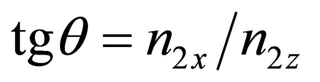 . For calculation of a trajectory of a ray it is necessary to substitute value tgθ, expressed through n2x, n2z in Equation (5). From Equation (10) also, as well as Equation (4) it is visible, that the component of a single vector along an axis z becomes zero in a ray’s turning points at
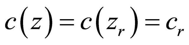 .
.
Thus, at analogy use between the description of propagation the sound along a ray and movement of a material particle (method 2) analytical expressions for components of a single vector along a trajectory of the ray, Equation (10), distinct from the expressions in Equation (3) received by method (1) with use of Snelius law, Equation (2), are received.
4. Calculation Ray’s Trajectories and Sound Field along Them with Two Methods
Let’s spend comparison two ways of ray’s trajectory calculation for a profile of a sound’s speed of a canonical form. We will accept, that the axis of the sound channel lays on depth of 1 km, depth of a waveguide is 4 km, the sound source is on a channel axis. It is easy to show, that ratio  is not a constant. However, calculation of this ratio for various rays shows, that it differs from a constant on small size. We will compare horizontal components of single vectors n1x, n2x trajectories of the rays, calculated under formulas (3) and (10). In Figure 1 values of n1x, n2x show as functions of depth z for the rays having turning points (ТP) below an axis of a wave guide on depths z1 = 1.75 km and z2 = 3.6905 km. In Figure 1 on a horizontal axis values n1x, n2x, are postponed, on vertical axis—depth z. In ТP
  all 4 curves have the identical values equal 1, n1x = n2x = 1, see Equations (3) and (10), on corresponding depths. Numbers 3,
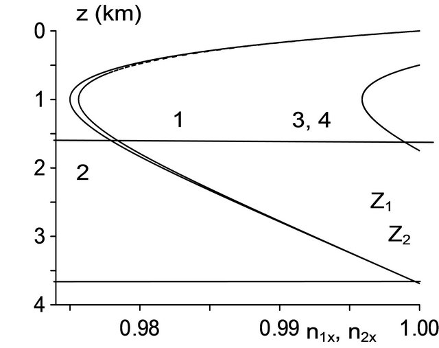
Figure 1. Dependence of projections of single vectors , from depth of a wave guide z for rays, curves 3, 4 with turning points at a bottom on depths z1 = 1.75 km and z2 = 3.6905 km, curve 1, 2, θ—an angle along a trajectory.
4 designate two curves coinciding on the scale of drawing having ТP on depth z1. Appreciable difference n1x, n2x is observed near to a wave guide axis, for steep rays, curves 1, 2,  , with ТP on depth z2. Figures in drawing near to these curves specify, what method calculates curves. Difference of curves is caused, obviously, not only distinction of the functions describing a ray trajectory (a vector n) in methods 1, 2, but also distinction of angles of departure at which rays have the same depth.
On Figure 2 the length of a cycle of rays as function of an angle of departure θ0, calculated in two methods is shown. The divergence of curves on the scale of drawing also is observed only for steep rays (the least θ0). The lower curve is calculated by a method 2, upper—on a method 1. It is visible, that length of cycle  (a method 1) more than that calculated by a method 2,
 . So, at depth of a tuning point a ray, z = 1.0005 km, angles θ0 coincide for two methods to within 5 th sign, a difference of cycle’s lengths
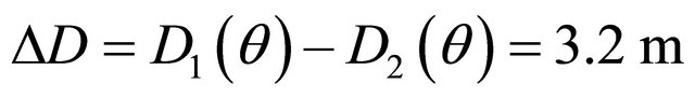 , at
, at
 .
.
Let’s consider vertical structure of a sound field z(θ) in the canonical wave guide, calculated in two ways. On Figure 3 angular distribution of vertical co-ordinates of the rays which have left a source towards a bottom, on distance from a source x = 500 km,  is resulted. An axis of abscises –angles of ray’s departure θ0, ordinate—depth z arrival of a corresponding ray on distance x from a source. An initial (greatest) θ0 = 89.998˚. Extremes of curves is co-ordinates of the caustic’s centers on depth on the given distance x. The continuous curve on Figure 3 is received by a method 1, shaped—a method 2. It is seen, that with decrease of a θ0 the curves coinciding at the big angles θ0, diverge a little, caustic’s co-ordinates do not coincide.
Similar curves with the caustic’s centers along an axis z only depending on time of arrival of rays, horizontal axis, are resulted in a number of works. On Figure 4 depth of
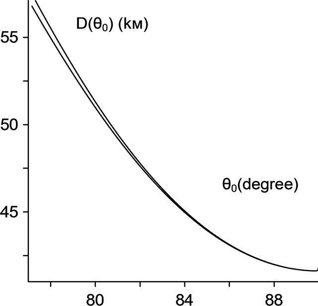
Figure 2. Dependence on an angle of departure of length of a ray’s cycle , calculated in two ways, the bottom curve —a method 2.
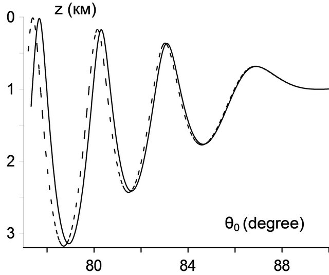
Figure 3. Angular distribution of vertical co-ordinates of rays at distance x = 500 km, calculated by two methods; a continuous curve—a method 1, shaped—a method 2, θ0—an angle of departure.
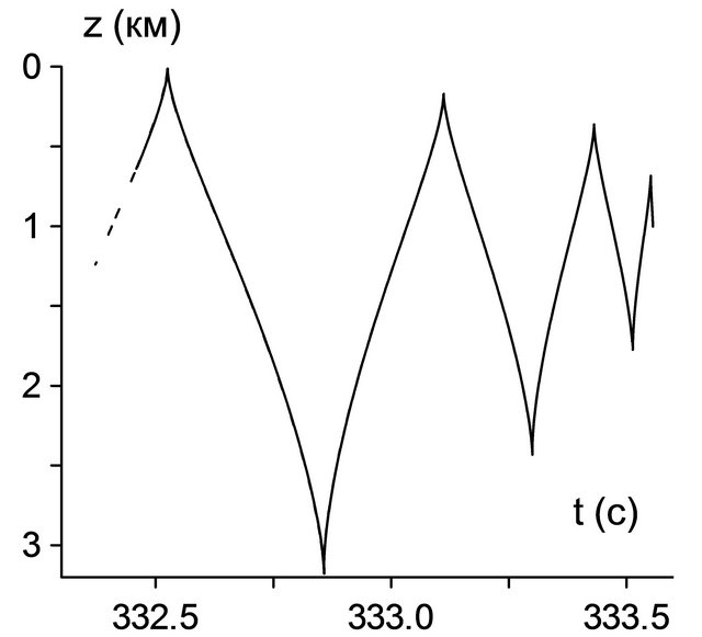
Figure 4. Vertical co-ordinates of rays as functions of time of arrival at distance x the = 500 km calculated by two methods; a continuous curve—a method 2, shaped—a method 1.
arrival’s rays which have left the source towards a bottom, depending on time of their propagation, horizontal axis, is shown. By a shaped line the co-ordinates of rays calculated by a method 2 are shown. Distinction of the curves is visible only in that range of time and depth, in which the rays calculated by a method 1, are absent. In other points curves on the scale of drawing coincide. In co-ordinates  the centers of caustics are tops of points of bend of curves
 . Comparison of numerical values of times of ray’s arrivals on the same depth shows, that times of propagation of the near horizontal rays, calculated by both methods, are very close to each other, considerable distinction is observed for steep rays. So, for corners θ ≥ 88˚ times of ray’s rrivals differ on ~ 1 - 3.10−4 c, time of arrival of the most steep rays calculated on a method 2 on ~ 0.3с more than calculated on method 1.
Let’s consider structure of the module of an acoustic field along a vertical, calculated by two methods, Figure 5, an abscise—an axis z, ordinate—the amplitude of field. The field calculates on frequency of 233.6 Hz. Continuous lines—calculation by a method 2, shaped—a method 1.
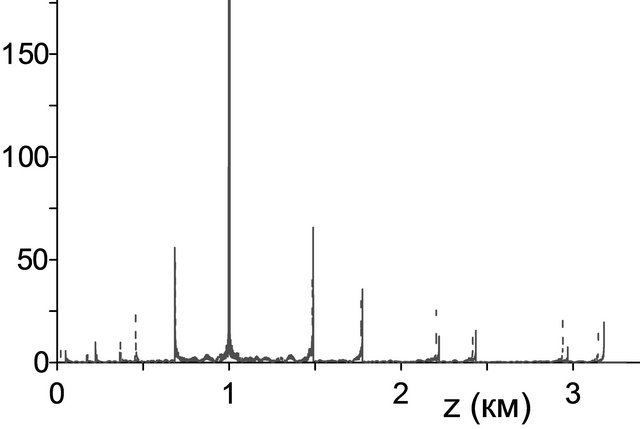
Figure 5. Structure of the module of an acoustic field along a vertical axis of a wave-guide at distance x = 500 km, calculated by two methods; a continuous line—a method 2, shaped—a method 1.
Distinction in caustic’s position and in value of amplitudes is visible.
5. Conclusions
As a result of comparison of two methods of obtaining of analytical expressions for a tangent to a ray trajectory, it is possible to draw the following conclusions. Practical coincidence of calculation of trajectories by two methods is the confirmation of legitimacy of the decision of a problem on sound propagation in the non-uniform space with the decision in ray approach. When the general structure of an acoustic field in a wave guide without quantitative comparison of separate characteristics is required, both methods of the account are equivalent. If it is necessary to compare calculated value with experiment, it is necessary to give preference to a traditional method 1. Under the physical concept, it is more proved than the 2nd method using formal analogy between action of a mechanical particle and eikonal of a sound wave.
The method of analogies is of interest as possibility of various comparisons by the nature of the physical phenomena, in which the general laws that promotes their deeper understanding can be found. In this case it is possibility to receive one more analytical expression for a tangent vector to a ray trajectory in approach of the geometrical acoustics, distinct from traditional, under Snelius’s law.
REFERENCES
- V. A. Zverev, V. P. Ivanov and G. K Ivanova, “Caustics in the Underwater Channel and Their Connection with the Wave-Front of Point Source,” Proceedings of the 13th L. M. Brekhovskikh’s Conference Ocean Acoustics, Moscow, 2011, pp. 49-52.
- V. A. Zverev, V. P. Ivanov and G. K Ivanova, “Caustics in the Underwater Channel and Their Connection with the Wave-Front of Point Source,” 2011. www.iapras.ru/publication/preprint/ca11.pdf/
- L. D. Landau and V. M. Lifshits, “Gidrodinamika,” Science, Мoscau, 1988.
- J. Simmen, S. M. Flatte and G.-Y. Wang, “Wavefront Folding, Chaos, and Diffraction for Sound Propagation through Ocean Internal Waves,” Journal of the Acoustical Society of America, Vol. 102, No.1, 1997, pp. 239-255. doi:10.1121/1.419820
- G. K. Ivanova, “Two Methods of Calculation of Sound Ray’s Trajectories at Ocean,” Proceedings of the 20th Conference of the Russian Acoustic Society, Moscow, 2008, pp. 338-341.
- G. J. Heard and N. P. Chapman, “Heard Island Feasibility Test: Analysis of Pacific Part Data Obtained with a Horizontal Line Array,” Journal of the Acoustical Society of America, Vol. 96, No. 4, 1994, pp. 2389-2394. doi:10.1121/1.410111
- L. D. Landau and V. M. Lifshits, “Mechanics,” PhysMath. Lit. State Publication, Moscau, 1958.
- V. I. Smirnov, “The Course of a Higher Mathematics,” Phys-Math. Lit. State Publ, Moscau, 1958.