Open Journal of Business and Management
Vol.06 No.01(2018), Article ID:80455,20 pages
10.4236/ojbm.2018.61001
Machine Learning Methods of Bankruptcy Prediction Using Accounting Ratios
Yachao Li, Yufa Wang
Henan Polytechnic University, Jiaozuo, Henan

Copyright © 2018 by authors and Scientific Research Publishing Inc.
This work is licensed under the Creative Commons Attribution International License (CC BY 4.0).
http://creativecommons.org/licenses/by/4.0/


Received: October 24, 2017; Accepted: November 18, 2017; Published: November 21, 2017
ABSTRACT
The aim of bankruptcy prediction is to help the enterprise stakeholders to get the comprehensive information of the enterprise. Much bankruptcy prediction has relied on statistical models and got low prediction accuracy. However, with the advent of the AI (Artificial Intelligence), machine learning methods have been extensively used in many industries (e.g., medical, archaeological and so on). In this paper we compare the statistical method and machine learning method to predict bankruptcy with utilizing China listed companies. Firstly, we use statistical method to choose the most appropriate indicators. Different indicators may have different characteristics and not all indicators can be analyzed. After the data filtering, the indicators are more persuasive. Secondly, unlike previous research methods, we use the same sample set to conduct our experiment. The final result can prove the effectiveness of the machine learning method. Thirdly, the accuracy of our experiment is higher than existing studies with 95.9%.
Keywords:
Bankruptcy Prediction, Statistical Method, Machine Learning, Accounting Ratios

1. Introduction
For a long time, corporate bankruptcy prediction is one of the utmost significance parts in evaluating the corporate prospects. Lenders, investors, governments and all kinds of stakeholders are eager to seek an efficient way to understand the ability of the company so that they can choose the suitable decision making. The whole condition of the corporate either small or large needs to develop the models to assess the financial risks. For example, Altman (1968), in a paper, used the multivariate discriminant analysis to predict the financial case [1] .
The original study in bankruptcy prediction can be dated back to the early 20th century when Fitzpatrick (1932) used economic index to describe predictive capacity of default business [2] . After that, more and more researchers focused on the bankruptcy prediction (e.g. Winakor and Smith(1935) [3] ; Merwin, (1942) [4] ). The turning point in the survey of the business failure symptoms was happened in 1966 by Beaver who initiated the statistical models to made financial forecasts. Following the line of thinking, there are many representative statistical models were proposed by scholars [5] . Ohlson (1980) used the logistic regression to forecast financial status [6] . Besides, in 1985, West determined financial forecasts with factor analysis [7] . Similar to the experiments, a great number of generalized liner models that can be used to predict financial conditions emerged continuously (e.g. Aziz, Emanuel and Lawson (1988) [8] ; Koh (2010) [9] ; Platt, Platt and Pederson (1994) [10] ; Upneja and Dalbor (2000) [11] ; Beaver, McNichols and Rhie(2005) [12] et al.).
From the beginning of the 20th century, AI and machine learning methods are becoming more popular in many different industries. For example, Subasai and Ismail Gursoy (2010) [13] and de Menezes, Liska, Cirillo, and Vivanco (2016) [14] in medicine; Maione et al. (2016) [15] and Cano et al. (2016) [16] in chemistry; Heo and Yang (2014) [17] in finance; Kim, Kang, and Kim (2015) [18] in finance. Except for those industries, it is widely used in a variety of discipline. Bankruptcy prediction is one of them. With the advent of the big data era, statistical models have some weaknesses in reflect bankruptcy prediction. Based on that, researchers have to find some new method to overcome the shortcoming of statistical method. Since the bankruptcy prediction is similar to the classify algorithm, academics are exploring machine learning tools can be used to separate bankruptcy and non-bankruptcy corporate (Wilson and Sharda (1994) [19] ; Tsai (2008) [20] ; Chen et al. (2011) [21] ). Besides, many researchers combine statistical methods and machine learning methods to enhance the reality of bankruptcy prediction continually. Cho et al. (2010) introduced the hybrid model by selecting variables filtered by decision tree and case-based reasoning using the Mahalanobis distance with weights [22] . Chen et al. (2009) introduced a hybrid model by combining the fuzzy logic and neural network [23] . The final results show that the hybrid model has a higher accuracy than logic model. All in all, with the development of information science, it has great influence on all fields of scientific research.
As a hot research topic in computer science, machine learning has many different components, which consists of the decision tree, support vector machines(SVM), K-nearest neighbor method (KNN), random forest, logistic regression , artificial neural network (ANN) and so on.
Support vector machines (SVM) are one of the most successful models, for example, Cortes and Vapnik (1995) [24] generate functions similar to discriminant analysis and final successful prediction of bankruptcy corporate. Except for this, there are many scholars using support vector machines (SVM) to recognize bankruptcy and non-bankruptcy as well (Shin et al. (2005) [25] ; Chaudhuri and De (2011) [26] ; Sun and Li (2012) [27] ). In order to improve the accuracy of bankruptcy prediction, many scholars try to change the algorithm. Chaudhuri and De (2011) choose fuzzy support vector machine to (FSVM) to solve the problem of bankruptcy prediction and they claimed the efficient of FSVM [26] . Zhou et al. (2009) proposed a direct method to optimize parameters in SVM [28] .
Artificial neural network (ANN) establishes an analogy with neural network. The model is a structure similar to the neural network. The input layer is the input variable and the output layer determines the output variables. Between the first layer and the final layer are hidden layers. Compared with the traditional statistical models, many non-linear relationships can be analyzed by using artificial neural network (ANN). Tsai (2014) introduced some machine learning method to predict bankruptcy and the final result show that the accuracy is 86% [29] . In a word, the artificial neural network (ANN) can improve the accuracy modify by setting the parameters. Based on that, the paper compares statistical methods and computer science methods to find the most effective bankruptcy prediction model.
The rest of papers proceed as follows. In Section 2, we briefly introduce the data filter processing methods and machine learning methods. In Section 3, we present the data filtering process. In Section 4, we do the experiment and display experiments result. Concluding the article and suggestions for the future research will be given in the last part of Section 5.
2. Methodology
2.1. Normal Distribution Test
Normal distribution is one of the components of hypothesis testing. The formula for one-dimension normal distribution is:
where is the mean or expectation of the distribution (and also its median and mode). is the standard deviation. is the variance.
According to the sample size, there are usually divide into two different categories:
1) If the number of samples is less than 2000, we will choose the shapiro-wilk test’s W-statistic to verify the normal distribution.
2) If the number of samples is more than 2000, we will choose the Kolmogorov-Smirnov test to verify the normal distribution. In this paper, our sample is less than 2000, so we are mainly to focus on the Shapiro-Wilk test.
The Shapiro-Wilk test is a test of normality in frequents statistics. The Shapiro-Wilk tests the null hypothesis that a sample came from a normally distributed population. The test statistic is:
where is the i-th order statistic, is the sample mean, the constants are given by
where and are the expected values of the order statistics of independent and identically distributed random variables sampled from the standard normal distribution, and is the covariance matrix of those order statistics.
2.2. Wilcoxon Rank-Sum Test
Wilcoxon rank-sum test is a non-parametric test. It does not require the assumption of normal distributions, so it is widely used in non-parametric test. It is as effective as the t-test in parametric test on parametric test. The basic idea for Wilcoxon rank-sum test was: if the test hypothesis was established, the rank and difference of the two groups were smaller. The Wilcoxon rank-sum test steps consist of the following three steps:
1) Establish hypothesis
H0: The overall distribution of the two groups was the same;
H1: The overall distribution of the two groups is different; the inspection level was 0.05.
Create two separate samples
The first sample size is , the second sample size is . In the capacity of the mixed sample (first and second), the sample ranksum is and the sample ranksum is .The value of Z is:
or
where
is the number of the subjects sharing rank;
is to modify the discrete variables.
According to the significance level, determine whether to accept the original hypothesis.
2.3. Principle Component Analysis (PCA)
Suppose that we have a random vector X:
With population variance-covariance matrix:
Consider the linear combinations:
Each of these can be thought of as a linear regression, predicting from . There is no intercept, but can be viewed as regression coefficients.
Note that is a function of our random data, and so is also random. Therefore it has a population variance.
Moreover, and will have a population covariance
Here the coefficients are collected into the vector
2.4. K Nearest Neighbors (KNN)
The principle idea of KNN is that if a majority of samples in the feature space in the k most adjacent samples belonging to a certain category, the sample also belong to this category. For example, in order to distinguish between cats and dogs, the circle and triangle are already classified by the two features of claws and sound, so what kind of star does this represent? The principle of KNN is shown in Figure 1(a) and Figure 1(b).
When k = 3, the three lines are the closest three points, so the circle is more, so the star belongs to the cat.
2.5. Logistic Regression
The logistic regression model is a two class model. It selects different features and weights to classify the samples, and calculates the probability of the samples belonging to a certain class with each log function. That is, a sample will have a certain probability, belong to a class, there will be a certain probability, belong to another class; the probability of large class is the sample belongs to the class.
2.6. Decision Tree
The decision tree is a predictive model that represents a mapping between object attributes and object values. It is classified according to the features, each node raises a problem, and the data are divided into two categories by judgment, and then continue to ask questions. These questions are learned from existing data, and when new data is added, the data can be partitioned into suitable leaves based on the tree’s problem.
2.7. Support Vector Machines (SVM)
Support vector machine (SVM) is a learning theory of VC dimension theory and structural risk minimization principle on the basis of statistics. According to the limited sample information in model complexity and learning ability, it will obtain the best generalization ability. SVM is a two classification algorithm, which can find a (N-1) dimension hyper plane in N dimension space. This hyper plane can classify these points into two categories. That is to say, if there are two classes of linearly separable points in the plane, SVM can find an optimal straight line separating these points.
2.8. Random Forest
Random forest is based on decision tree. It is a classifier that combines existing classifiers algorithms in a certain way to form a classifier with stronger

Figure 1. The principle of KNN.
performance, and a weak classifier is assembled into a strong classifier. Its algorithm process is as follows:
1) Extract training sets from the original sample set. Each round extracts N training samples from the original sample using Bootstraping (In the training set, some samples may be extracted several times, while some samples may not be extracted at one time). K rounds were extracted and k independent training sets were obtained;
2) K decision tree models are obtained through K training sets;
3) K decision tree model is adopted to get the classification results by voting. the importance of all models is the same.
3. Data Selection
3.1. Data-Set
In this paper, the data set is collected from the Wind Financial Terminal Database and CCER Economic and Financial database. It contains all kinds of financial data of capital market enterprises which being disclosed by the financial statements. In China, if the listed company loses two consecutive years, it will be marked ST. In addition, the company that has been losing money for three years will be marked *ST. Such companies would be in danger of exiting the capital markets. In order to assess the reliability of the method, we are going to draw random sampling financial data covering 2000 to 2016 on China capital market companies. In this paper, we will take the company of ST as the bankruptcy sample and the company of net profit for four years is positive as the non-bankruptcy sample. The process of data selection follows the following proceeds:
First of all, in China, financial industry and non-financial industry follows the different accounting standards. So there are some differences in accounting statements and we need to distinguish two kinds of industry. However, financial industry have too much uncertainty mainly based on the national policies and regulations, so it has the high risk, therefore we decided to analyze non-financial industry.
Next, it is necessary to choose the indicators to evaluate the enterprise. From the financial management perspective, the enterprise evaluation mainly consists of the following four abilities: Debt Paying ability, Operation ability, Profit ability and Development ability. Moreover, different ability measurement system has different index composition. The indicators considered in the paper are described in details in Table 1. After the above steps, 518 companies are selected as samples. The numbers of observation in each year are shown in Table 2.
3.2. Data Filtering Results
To reduce the computational complexity and improve the significance of the model, it is necessary to make a significance test and filter candidate indicator variables. The proceeds of filter are as follows:
Before the significance test, the normal test of each indicator is required. We need to determine which method to perform the significance test according to

Table 1. The set of indicators considered in classification process.
the normal distribution test results. If the variable obeys the normal distribution, the appropriate indicators are selected according to T-test method. On the contrary, if the variable does not obey the normal distribution, we need to calculate
Table 2. The number of observations of different types of samples in each observed years.
Wilcoxon rank and perform non-parametric test. In the end, according to the standard of certain significance level, the model variables will be determined. In this paper, stata 10.0 is selected as the data statistics software. Stata is widely used in data analysis and it provides everything researchers need for statistics, graphics, and data management.
There are many methods to check the normal distribution. Different methods apply to different sample characteristic. Based on the sample of the paper, we choose Shapiro-Wilk test as a method. Shapiro-Wilk test is applicable to normal distribution test of sample size less than 2000. Besides, it is widely used in explore the distribution of continuous random variables. The selected financial indicators are inspected and the results are shown in the Table 3.
Table 3 list the test results of the sample. In the Table 3, Obs on behalf of the number of the samples. In this paper, the number of all variables is 518, so the value of Obs is 518. W; V and z are intermediate variable of normal test. According to the determination principle, the final result will be determined by the P value (Prob > z). In mathematical statistic hypothesis, all the test indicators are subject to normal distribution. But the P value (Prob > z) is the basis for judging whether to accept the original hypothesis. If P value is less than 0.05, we need to accept the original hypothesis. It means that all of the variables are in a normal distribution. However, if P value is greater than 0.05, it is necessary to reject the original hypothesis and we assume that the variables don’t fit the normal distribution. According to the above decision principle, the P value of all variables is
Table 3. Normal distribution test results.
less than 0.05, so we can make a decision that all indicators are not subject to normal distribution. After the normal distribution test, the difference significance test method should be selected according to the test results. The normal test results of this paper can be seen that all indicators require non-parametric test. The test results are shown in the Table 4.
As for non-parametric test of financial indicators, we select the Wilcoxon rank-sum test methods .The Wilcoxon rank-sum test is used for the two kinds of classification non-parameter test. Similar to the Shapiro-Wilk test, we need to eliminate the untested financial indicators based on the P value. If P value is less than 0.05, we need to accept the indicators. On the contrary, if P value is greater than 0.05, it is necessary to eliminate indicators. From the Table 4, the C1 and C2 P values of operating capability financial indicators are 0.7584 and 0.7912 respectively. Besides, the D6 index of development ability is 0.5746. The above three indexes are all greater than 0.05, so they are not tested by non-parametric and need to be eliminated. The P value of the remaining indicators is less than
Table 4. Non-Parametric test results.
0.05, so the financial indicators can be distinguished significantly and needs to be retained as the test financial indicator. Through the above index analysis process, the final selected sample index is A1. A2 and A3 in Profit ability, B1. B2. B3. B4 and B5 in paying ability, C3. C4 and C5 in operation ability, D1. D2. D3. D4. D5. D7. D8 and D9 in development ability.
4. Experiments
After data filtering, it is necessary to conduct the experiment. In this section, we will take both statistical and machine learning methods to predict bankruptcy. Figure 2 illustrates our methodology.
In this paper 19 variables are selected, it can be merged into profit ability, paying ability, operation ability and development ability. We will use 518 companies to complete bankruptcy prediction in two ways. The first way is statistical method. We plan to use logistic regression to conduct the experiment. The second way is machine learning method. Machine learning methods need to

Figure 2. The structure of this paper.
train data, so we will choose the proper train set. After the process of learning, we will take test set to complete bankruptcy prediction. After the experiment, we will compare the accuracy of two methods and determine which method is more accurate.
4.1. Statistical Method
In this section, we will take statistical method to conduct bankruptcy prediction. The bankruptcy prediction of statistical methods is mainly composed of the following steps: Firstly, it is necessary to analyze the principal component of four financial analysis indicators. Secondly, the binary logistic regression analysis is used to predict the bankruptcy. The results of Principle Components Analysis can be seen in Table 5.
In this section, we conducted principal component analysis on four financial indicators. After principal component analysis, we extracted the first principal components as a comprehensive evaluation of each financial index. During the period of principle component analysis, the gravel figure, score figure and loading figure of each variable are shown in Figure 3.
Figure 3 shows the gravel figure, score figure and loading figure of each variable. Loading figure in Figure 3(a) shows that two principal components of profit ability emphasis on different financial indicators. As for the first
Table 5. The results of principal component analysis.
components, V1 plays a major part and V2 plays the weakest role. From the gravel figure, we can see that eigenvalues greater than 1 consists of the first principal component and the second principal component. Therefore, according to the above analysis, we select the first principal component as an indicator of profit ability. Based on the above analysis process, we confirm that the first principal component is used as a measure of paying ability. Operation ability and development ability. After the dimension reduction of various financial indicators, four comprehensive abilities are formed to measure four financial indicators, respectively F1 F2 F3 and F4 the comprehensive evaluation ability of each financial index is as follows:
where
F1 is the comprehensive evaluation of profit ability;
F2 is the comprehensive evaluation of paying ability;
 (a)
(a) (b)
(b) (c)
(c)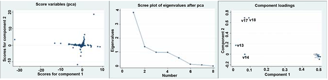 (d)
(d)
Figure 3. The gravel figure, score figure and loading figure of each variable. (a) Profit ability; (b) Paying ability; (c) Paying ability; (d) Development ability.
F3 is the comprehensive evaluation of operation ability;
F4 is the comprehensive evaluation of development ability.
After principal component analysis, we reduced our 19 financial measures to 4 financial indicators. Based on that, we perform binary logistic regression on F1 F2 F3 and F4 respectively. The results of bankruptcy prediction can be seen in Table 6.
From Table 6, we can draw the following conclusions: The Non-bankruptcy prediction probability of the enterprise is 86% and bankruptcy prediction probability of the enterprise is 55.8%. Therefore, the probability of accurate prediction is 70.8%. This probability is consistent with the exact probability of the most financial model predictions. However, the prediction accuracy of this model is not high and needs to be improved.
4.2. Machine Learning Methods
After the statistical method, we will take machine learning methods to take bankruptcy prediction. In this section, we choose KNN. SVM. Logistic regression. Random forest and decision tree to forecast bankruptcy. Figure 2 shows the ROC (Receiver Operating Characteristic) curve of random forest model.
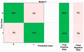
From Figure 4, we can draw the conclusion that random forest model shows the outstanding accuracy. The square of the shaded area has reached 0.99, which is close to the largest area 1. The shaded area shows the diagnosis effect. The bigger the shadow, the better the diagnosis effect. Besides, in order to verify the effectiveness of more machine learning methods, we enumerated the confusion matrix of five machine learning methods. The confusion matrix of five machine learning methods can be seen in Figure 5.
Figure 5 shows the bankruptcy prediction outcomes for machine learning methods. The random forest and decision tree shows high accuracy with 95% and 94% in non-bankruptcy prediction. Besides, the KNN. SVM and logistic regression have the lower accuracy with 88% 88% and 84% respectively. However, compared to statistical method with 86%, four machine learning methods have the higher predictive accuracy except for logistic regression. As for bankruptcy prediction, machine learning methods show significant superiority over statistical method. The random forest shows the highest accuracy with 97% and the KNN shows the lowest accuracy with 74% which is much greater than statistical method with 55.8%. In addition, the remaining fours machine learning methods also have high prediction accuracy than statistical method.
In conclusion, the machine learning method has the higher bankruptcy prediction accuracy than statistical method. Overall results of different methods can be seen in Figure 6. The prediction of random forest is 95.9%. It is clear that
Table 6. The results of bankruptcy prediction.

Figure 4. ROC curve of random forest model to predict bankruptcy, with data from China capital market listed companies.
 (a)
(a)
 (b)
(b)
 (c)
(c)
 (d)
(d)
 (e)
(e)
Figure 5. Confusion matrix of each machine learning method. (a) Bankruptcy prediction of KNN; (b) Bankruptcy prediction of SVM; (c) Bankruptcy prediction of Logistic R; (d) Bankruptcy prediction of Random Forest; (e) Bankruptcy prediction of Decision Tree.

Figure 6. Overall results of different methods.
machine learning method is more accurate than other prediction method. The results demonstrate that machine learning method has the advantage to predict bankruptcy over the statistical method.
5. Conclusions
This paper compares the accuracy of statistical forecasting and machine learning methods to predict bankruptcy in Chinese-listed companies. Firstly, we take Shapiro-Wilk test to test the normal distribution. Secondly, according to the Shapiro-Wilk test result, it is necessary to determine the parameter test or the non-parametric test. In the end, we take both statistical method and machine learning method we predict bankruptcy. The empirical results show that machine learning methods are superior to statistical methods.
As for statistical method, we choose principal component analysis to reduce the 19 financial statements to 4 financial indicators. Through a comprehensive measurement of financial indicators, we carry out binary logistic regression to four comprehensive indexes. The final rate of accuracy is 70.8%. However, each machine learning method (KNN, SVM, Logistic Regression, Decision Tree, and Random Forest) has the greater accuracy than statistical method.
In the future, we plan to extend our work to more indicators of the companies. With the development of the China capital market, there will be more company characteristics to be disclosure. Based on this trend, we will select more indicators to predict bankruptcy. Furthermore, we will apply the method to more small and medium enterprise in China. Subsequently, we would try more machine learning method and improve the accuracy of bankruptcy prediction.
Cite this paper
Li, Y.C. and Wang, Y.F. (2018) Machine Learning Methods of Bankruptcy Prediction Using Accounting Ratios. Open Journal of Business and Management, 6, 1-20. https://doi.org/10.4236/ojbm.2018.61001
References
- 1. Altman, E.I. (1968) Financial Ratios, Discriminant Analysis and the Prediction of Corporate Bankruptcy. Journal of Finance, 23, 589-609. https://doi.org/10.1111/j.1540-6261.1968.tb00843.x
- 2. Fitzpatrick, P.J. (1932) A Comparison of the Ratios of Successful Industrial Enterprises with Those of Failed Companies. Análise Molecular Do Gene Wwox, 598-605.
- 3. Smith, R. and Winakor, A. (1935) Changes in the Financial Structure of Unsuccessful Corporations.
- 4. Merwin, C.L. (1942) Financing Small Corporations in Five Manufacturing Industries, 1926-1936: A Dissertation in Economics. Financing Small Corporations in Five Manufacturing Industries, 1926-36. National Bureau of Economic Research.
- 5. Beaver, W.H. (1966) Financial Ratios as Predictors of Failure. Journal of Accounting Research, 4, 71-111. https://doi.org/10.2307/2490171
- 6. Ohlson, J.A. (1980) Financial Ratios and the Probabilistic Prediction of Bankruptcy. Journal of Accounting Research, 18, 109-131. https://doi.org/10.2307/2490395
- 7. West, R.C. (1985) A Factor-Analytic Approach to Bank Condition. Journal of Banking & Finance, 9, 253-266. https://doi.org/10.1016/0378-4266(85)90021-4
- 8. Aziz, A., Emanuel, D.C. and Lawson, G.H. (1988) Bankruptcy Prediction—An Investigation of Cash Flow Based Models. Journal of Management Studies, 25, 419-437. https://doi.org/10.1111/j.1467-6486.1988.tb00708.x
- 9. Koh, H.C. and Killough, L.N. (2010) The Use of Multiple Discriminant Analysis in the Assessment of the Going-Concern Status of an Audit Client. Journal of Business Finance & Accounting, 17, 179-192. https://doi.org/10.1111/j.1468-5957.1990.tb00556.x
- 10. Platt, H.D., Platt, M.B. and Pedersen, J.G. (1994) Bankruptcy Discrimination with Real Variables. Journal of Business Finance & Accounting, 21, 491-510. https://doi.org/10.1111/j.1468-5957.1994.tb00332.x
- 11. Upneja, A. and Dalbor, M.C. (2000) An Examination of Capital Structure in the Restaurant Industry. International Journal of Contemporary Hospitality Management, 13, 54-59. https://doi.org/10.1108/09596110110381825
- 12. Beaver, W.H., Mcnichols, M.F. and Rhie, J.W. (2005) Have Financial Statements Become Less Informative? Evidence from the Ability of Financial Ratios to Predict Bankruptcy. Review of Accounting Studies, 10, 93-122. https://doi.org/10.1007/s11142-004-6341-9
- 13. Subasi, A. and Gursoy, M.I. (2010) Eeg Signal Classification Using pca, ica, lda and Support Vector Machines. Expert Systems with Applications, 37, 8659-8666. https://doi.org/10.1016/j.eswa.2010.06.065
- 14. Menezes, F.S.D., Liska, G.R., Cirillo, M.A. and Vivanco, M.J.F. (2016) Data Classification with Binary Response through the Boosting Algorithm and Logistic Regression. Expert Systems with Applications, 69, 62-73. https://doi.org/10.1016/j.eswa.2016.08.014
- 15. Maione, C., Paula, E.S.D., Gallimberti, M., Batista, B.L., Campiglia, A.D., Jr, F.B., et al. (2016) Comparative Study of Data Mining Techniques for the Authentication of Organic Grape Juice Based on icp-ms Analysis. Expert Systems with Applications, 49, 60-73. https://doi.org/10.1016/j.eswa.2015.11.024
- 16. Cano, G., Garcia-Rodriguez, J., Garcia-Garcia, A., Perez-Sanchez, H., Benediktsson, J.A., Thapa, A., et al. (2016) Automatic Selection of Molecular Descriptors using Random Forest: Application to Drug Discovery. Expert Systems with Applications.
- 17. Heo, J. and Yang, J.Y. (2014) Adaboost Based Bankruptcy Forecasting of Korean Construction Companies. Applied Soft Computing, 24, 494-499. https://doi.org/10.1016/j.asoc.2014.08.009
- 18. Kim, M.J., Kang, D.K. and Hong, B.K. (2015) Geometric Mean Based Boosting Algorithm with Over-Sampling to Resolve Data Imbalance Problem for Bankruptcy Prediction. Expert Systems with Applications, 42, 1074-1082. https://doi.org/10.1016/j.eswa.2014.08.025
- 19. Wilson, R.L. and Sharda, R. (1994) Bankruptcy Prediction Using Neural Networks. Decision Support Systems, 11, 545-557. https://doi.org/10.1016/0167-9236(94)90024-8
- 20. Tsai, C.F. (2008) Financial Decision Support using Neural Networks and Support Vector Machines. Expert Systems, 25, 380-393. https://doi.org/10.1111/j.1468-0394.2008.00449.x
- 21. Chen, M.Y. (2011) Predicting Corporate Financial Distress Based on Integration of Decision Tree Classification and Logistic Regression. Expert Systems with Applications, 38, 11261-11272. https://doi.org/10.1016/j.eswa.2011.02.173
- 22. Cho, S., Hong, H. and Ha, B.C. (2010) A Hybrid Approach Based on the Combination of Variable Selection using Decision Trees and Case-Based Reasoning using the Mahalanobis Distance: For Bankruptcy Prediction. Expert Systems with Applications, 37, 3482-3488. https://doi.org/10.1016/j.eswa.2009.10.040
- 23. Chen, H.J., Huang, S.Y. and Lin, C.S. (2009) Alternative Diagnosis of Corporate Bankruptcy: A Neuro Fuzzy Approach. Expert Systems with Applications, 36, 7710-7720. https://doi.org/10.1016/j.eswa.2008.09.023
- 24. Cortes, C. and Vapnik, V. (1995) Support-Vector Networks. Machine Learning, 20, 273-297. https://doi.org/10.1007/BF00994018
- 25. Shin, K.S., Lee, T.S. and Kim, H.J. (2005) An Application of Support Vector Machines in Bankruptcy Prediction Model. Expert Systems with Applications, 28, 127-135. https://doi.org/10.1016/j.eswa.2004.08.009
- 26. Chaudhuri, A. and De, K. (2011) Fuzzy Support Vector Machine for Bankruptcy Prediction. Applied Soft Computing Journal, 11, 2472-2486. https://doi.org/10.1016/j.asoc.2010.10.003
- 27. Sun, J. and Li, H. (2012) Financial Distress Prediction using Support Vector Machines: Ensemble vs. Individual. Applied Soft Computing Journal, 12, 2254-2265. https://doi.org/10.1016/j.asoc.2012.03.028
- 28. Zhou, L., Lai, K.K. and Yu, L. (2009) Credit Scoring using Support Vector Machines with Direct Search for Parameters Selection. Soft Computing, 13, 149. https://doi.org/10.1007/s00500-008-0305-0
- 29. Tsai, C.F., Hsu, Y.F. and Yen, D.C. (2014) A Comparative Study of Classifier Ensembles for Bankruptcy Prediction. Applied Soft Computing, 24, 977-984. https://doi.org/10.1016/j.asoc.2014.08.047