Theoretical Economics Letters
Vol. 2 No. 1 (2012) , Article ID: 17347 , 9 pages DOI:10.4236/tel.2012.21001
Spatio-Temporal Patterns for a Generalized Innovation Diffusion Model
1College of Management of Technology, Swiss Federal Institute of Technology, Lausanne, Switzerland
2School of Engineering, Laboratory of Microengineering for Manufacturing, Swiss Federal Institute of Technology, Lausanne, Switzerland
3Mathematical and Computational Sciences Department, IBM Zurich Research Laboratory, Rueschlikon, Switzerland
Email: fariba.hashemi@epfl.ch
Received October 18, 2011; revised November 15, 2011; accepted December 25, 2011
Keywords: Diffusion of innovation; Bass’ model; interactive multi-agent systems; local interactions; imitation processes; stochastic dynamics; alternating renewal processes; mean-field dynamics; discrete velocity collisions models; nonlinear field equations; exact transient evolutions
ABSTRACT
We construct a model of innovation diffusion that incorporates a spatial component into a classical imitation-innovation dynamics first introduced by F. Bass. Relevant for situations where the imitation process explicitly depends on the spatial proximity between agents, the resulting nonlinear field dynamics is exactly solvable. As expected for nonlinear collective dynamics, the imitation mechanism generates spatio-temporal patterns, possessing here the remarkable feature that they can be explicitly and analytically discussed. The simplicity of the model, its intimate connection with the original Bass’ modeling framework and the exact transient solutions offer a rather unique theoretical stylized framework to describe how innovation jointly develops in space and time.
1. Introduction
Since the middle of the XXth century, a substantial literature emphasizes the importance of quantitative models that enable the forecasting of the diffusion of technological innovations (DTI) not only for pure academic interest, but for its practical relevance. While the empirical evidence that quantification of DTI is possible was initially recognized by E. Mansfield [1] and Z. V. Griliches [2,3], the first quantitative stylized dynamical modeling framework was proposed by F. Bass in his seminal 1969 paper [4]. Similar in essence to the P.-F. Verhulst’s epidemiological logistic equation, the Bass’ model uses an aggregated differential approach enabling the reproduction of the relevant dynamical features of the adoption of a new product and/or a new technology in a society of consumers. Bass’ nonlinear dynamics is basically governed by the ratio of two control parameters, namely the innovation and imitation rates. Introducing a quadratic nonlinearity into the evolution equation, the model mathematically describes consumer imitative interactions. This nonlinearity leads to an evolution characterized by two distinct time scales, i.e. a fast initial exponentially growing phase followed by a slow asymptotic evolution when full equilibrium demand is nearly reached. The seminal works of J. A. Schumpeter [5] and subsequently of B. Jovanovic and R. Rob [6] support this observation by illustrating the importance of imitation waves in DTI and the formation of business cycles.
In general, interaction-based models have been employed for various applications ranging from epidemiology [7], variance of crime rates across space when direct interdependencies occur between nearest neighbors [8], herd behavior in financial markets [9-12] to social movements and political uprisings (see [13] and [14] for several additional references). Interaction-based methods have also been useful tools in modeling the diffusion of innovation [16-21]. In their contribution, G. Ellison and D. Fudenberg [22,23] study agents who consider the experiences of their neighbors in deciding which of two technologies to adopt, in a world where players use rules of thumb that ignore historical data but may incorporate a tendency to use the more popular technology. In this learning environment, agents observe both their neighbors’ choices, and periodically reevaluate their decisions, as opposed to making a once-and-for-all choice. R. Andergassen et al. [24] investigate the evolutionary process of imitation and innovation as a search mechanism in a given neighbourhood of firms. In their world, the spreading of information through neighbourhoods allows firms to acquire knowledge leading to innovation waves as firms attempt to glean information on best practice techniques, which they subsequently imitate. For additional models where preference orderings over alternatives in a choice set can depend on the actions chosen by other agents, see [25-28].
The original Bass’ dynamics is aggregated and hence fails to detail the influence of spatial location of agents in the imitative behavior of consumers. Intuitively, spatial considerations strongly affect the interactions between agents and the underlying imitation mechanisms. In fact spatial proximity is argued to be a major driving force of innovation diffusion which often exceeds the external marketing efforts such as advertising [29,30]. In 1991, P. Krugman [31] pointed out that production is remarkably concentrated in space. This observation opened a strong research effort devoted to the understanding of the spatial dimension of innovation diffusion. M. P. Feldman [32,33] echoed P. Krugman’s observation in pointing out that geographical effects are even more stringent for innovative activity because the rationale for the formation of adopter clusters is related to the role of word-of-mouth and imitation in the diffusion of innovations. As emphasized in [34], a clear correlation exists between geographical proximity and the strength and speed of word-of-mouth spread, sometimes labeled as the neighborhood effect.
In addition to these works, a wealth of empirical studies exemplify the importance of geography in the diffusion of knowledge and R & D. Spatially-mediated knowledge spillovers of R & D are explicitly discussed in [35- 38]. It is noteworthy to observe that this pure geographic view can be generalized by defining metric distances on abstract state spaces in order to describe the evolution of technological advance, R & D investment volume or any other abstract features [39] on which agents can compete by adjustment of their individual behavior.
Recent literature suggests that imitation interactions between interacting agents like bacteria, flies, quadrupeds or fishes can explain the formation of compact spatio-temporal patterns, i.e. swarms or platoons, which spatially evolve as quasi-solid bodies [40,41]. The flocking mechanism originates from mimetic type decisions based on agents’ observations of their neighbors. To the best of our knowledge, spatial flocking mechanisms seem to be barely discussed in the interaction-based socioeconomic literature. Hence a natural and simple attempt to analytically infer the role of spatial parting is to introduce spatial effects and it is the aim of our paper to incorporate their influence into the original Bass’ evolution.
Adding a spatial dimension transforms the Bass’ ordinary differential equation into a partial differential equation (PDE). Due to the underlying imitation mechanism, the resulting PDE will be intrinsically nonlinear, a perspective that generally offers little hope for explicit solutions in the realm of field theories. The present paper illustrates how a simple natural spatial extension of the original Bass’ dynamics leads nevertheless to a fully solvable nonlinear field dynamics, a truly remarkable result. The resulting equations belong to the discrete velocities Boltzmann equations (DVBE) which describe the macroscopic properties of a dilute gas. The specific DVBE that can be derived from the Bass’ dynamics coincide with the Ruijgrok-Wu (RW) model introduced and solved by T. W. Ruijgrok and T. T. Wu [42]. This intimate connection with statistical physics suggests that the Bass’ dynamics can be obtained, via a mean-field limit, from a microscopic point of view in which a large number of agents interact. While the mean-field approach is a basic tool in statistical physics of large systems, it has now been explicitly used in recent econometric studies as well (see illustrations in [10-12,14,15,28]). Relying on the law of large numbers, the mean-field limit allows one to write deterministic evolution for probability densities in question. In the sequel, we will explicitly construct the microscopic connection that exists between the Bass’ imitation model with spatial effects and the RW model inspired by a similar approach adopted in [43] for a multiagent dynamics in logistics and econophysics contexts. In [43], the dynamics exhibit a nonlinear term due to a specific imitation mechanism giving rise to the famous Burgers’ nonlinear PDE to describe the emergence of spatio-temporal patterns. As illustrated in [44], RW dynamics actually generalizes the Burgers’ equation, the spatio-temporal Bass’ model presented here can itself be viewed as a natural generalization of the multi-agent imitation model studied in [43].
Besides its direct practical relevance, the simplicity of the original Bass model, for which exact analytical solutions are available, has undoubtedly contributed to its popularity in the economics and management literatures. Endowing Bass’ dynamics with spatially-dependent imitation mechanisms confers a new dimension to interaction-based socioeconomic modeling, opening the possibility to analytically study the generation of spatio-temporal patterns in a highly nonlinear context. Our stylized dynamics can be viewed as an exceptional possibility to analytically observe the spatio-temporal effects arising for a collection of agents subject to imitation interactions.
2. Spatially-Dependent Imitation Dynamics
Consider a collection  of N autonomous agents which are in a migration process on the one-dimensional real line
 . At any time
 , we assume that the complete population is composed by two types of agents
  and
and ,
,  , characterized by two associated
  -dependent migration velocities
  and
and  on
on . At any time, each agent is subject to modify his/her velocity. Agents
 ,
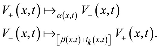
,  , change their velocity either spontaneously or after an autonomous decision based on an imitation process (IP). Let us write
 , respectively
 , as the spontaneous transformation rates from states
 , respectively
 . Apart from these spontaneous transitions, additional transitions are assumed to be triggered by mutual agents’ interactions. Specifically, for an agent
 , located at position x at time
 , the IP mechanism is assumed to depend on the observation of the current velocity states, (i.e.
  or
or ), adopted by other proximity members located in the neighborhood
  of agent
  (by neighborhood
  we assume here a linear interval around the location x of agent
 , it will be further defined in Equation (5)). For an arbitrary agent
 , we define his/her imitation decision rule according to his/her interactions with other agents as follows:
1) Dynamic rule for an agent . At time
 , the agent
  simultaneously observes the (velocity) state of the agents contained in his/her neighborhood
  The presence of agents
 ,
,  , seen by
  triggers an imitation mechanism which enhances the transition rate towards the state
 , i.e.
  The extra contribution
  is proportional to (i.e. is monotonically increasing with) the number of agents
 ,
,  , in the neighborhood
  of agent
 .
.
2) Dynamic rule for an agent . At time
  the agent
  simultaneously observes the (velocity) state of the agents contained in his/her neighborhood
  and does not modify its velocity whatever he/she observes.
According to these dynamic rules, the time-dependent position  of agents
 ,
,  , can be written as a set of coupled stochastic differential equations (SDEs):
 (1)
(1)
where  stands for a two-velocity-states Markov chain (i.e. the state space is here
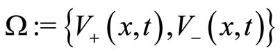 ), the transition rates of which are defined by:
 (2)
(2)
The noise source in Equation (1) can also be viewed as a non-homogeneous, alternating, Markov renewal process in which the inverse transition rates  and
and  are respectively the mean sojourn times in states
  and
and . We can therefore directly observe that in Equation (1), the coupling between the various agents is realized via the extra
  transition rate.
For an agent , located at position x at time
 , we shall write:
 (3)
(3)
where  is the neighborhood affecting the imitation rate of agent
 , and
, and  stands for the indicator function. From now on, we consider a very large population of agents, i.e.
 , and instead of individual agent trajectories, we now think in terms of probability densities in order to characterize the evolution of the global population
  of agents. To this aim, we write
  and
and  to denote the density of agents
  and
and  to be found at position
  at time
 .
.
For such a large population of agents, individual fluctuations become negligible and we can adopt a meanfield approach (MFA). This consists in considering that, statistically, the time evolution of an arbitrary agent is representative of the whole population. When this representative agent is located at position x at time , the MFA views the influence of other agents inside his/her neighborhood
  as an external effective interactive mean-field which enables us to replace Equation (1) by a single scalar SDE:
 (4)
(4)
where in Equation (4), the  transition rates are replaced by an effective rate
  defined by:
 (5)
(5)
where the radius  characterizes the size of the neighborhood interval
  which triggers the IP of the representative agent. Note that for diffusion processes, SDEs of the type given by Equation (1), driven by WGN, have been recently used for describing multi-agent dynamics with IP in [43]. In this particular situation, the rigorous mathematical foundations for the MFA procedure have been established in [45].
Associated with the SDEs given by Equations (4) and (5), the MFA enables us to write a Fokker-Planck equation for the probability densities  and
and , [44]:
 (6)
(6)
where the imitation rate term in Equation (6) reads as:
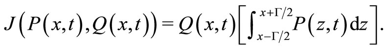 (7)
(7)
The dynamics in Equation (6) is a coupled set of nonlocal and nonlinear field equations, which barely offers hope for any analytical discussion. However, for small radius  (i.e. infinitesimal interaction neighborhoods), we may Taylor expand Equation (6), up to first order in
 , to obtain:
 (8)
(8)
We directly observe that Equation (8) can be viewed as a generalized Bass’ dynamics which confers relevance to the spatial dimension on which agents evolve. Indeed, similarly to the original Bass’ model, we include an imitation process, represented in Equation (8) by the nonlinear contribution .
.
Writing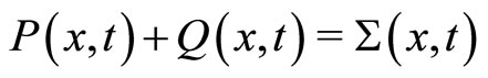 , the summation of both equations in (8) yields a continuity equation:
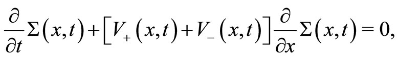 (9)
(9)
which in turn implies the normalization constraint:
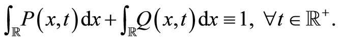 (10)
(10)
Although the dynamics given by Equation (8) has been derived for non-homogeneous and non-stationary parameters ,
,  and
and , in the sequel we will restrict our attention to situations where these parameters can be assimilated to constants (i.e.
  and
and ).
).
Spatial Homogeneous Regimes—Bass’ Model
When , the spatial character disappears from the dynamics given by Equation (8), which implies that
  and
and  More precisely, Equation (8) becomes:
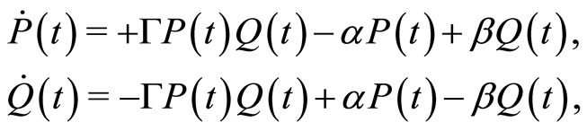 (11)
(11)
with the notation . The constraint given by Equation (10) now simply becomes
  and enables us to rewrite Equation (11) in the following form:
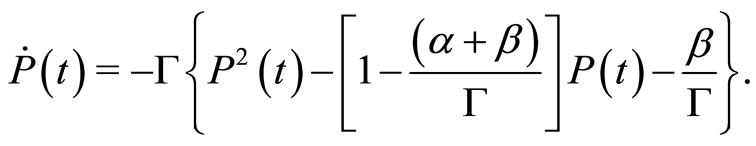 (12)
(12)
At this stage, it is worth observing that for  and
and , Equation (12) reduces to
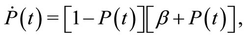 (13)
(13)
which is precisely the original Bass’ dynamics [4] with  being the ratio between the imitation and innovation rates.
For completeness of the exposition, let us integrate Equation (12), with the initial condition , to get:
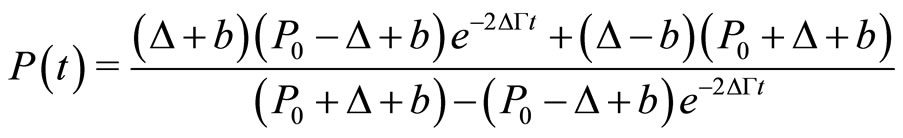 (14)
(14)
with the definitions:
 and
and 
In the asymptotic time limit , Equation (14) converges to:
 (15)
(15)
For the original Bass’ model obtained when 
and , we have
  and
and .
.
Accordingly, with , Equation (14) reduces to the original Bass’ solution:
 (16)
(16)
Moreover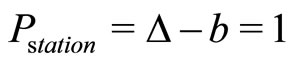 , which expresses the fact that all agents ultimately adopt the new technology, as it is obviously expected in the original Bass’ modeling framework, when
 .
.
3. Bass’ Dynamics with Spatio-Temporal Effects
Coming back to the dynamics given by Equation (8) and introducing dimensionless coordinates via the Galileo transformation 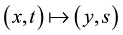 defined by:
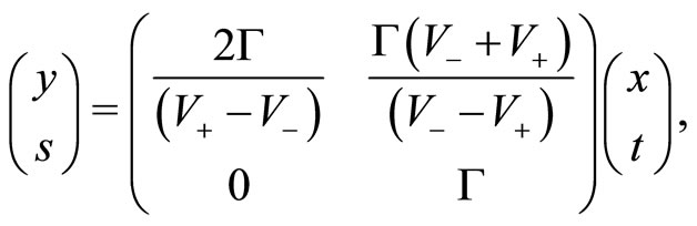 (17)
(17)
we straightforwardly have:
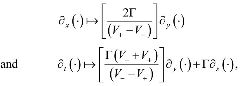 (18)
(18)
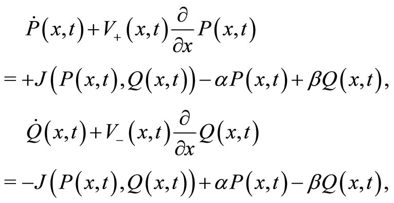
which transforms Equation (8) into the coupled set of nonlinear partial differential equations (PDEs):
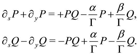 (19)
(19)
The set of non-linear PDEs given by Equation (19) can be interpreted as being a discrete two velocity model of Boltzmann equations, first studied in [42]. The dynamics given by Equation (19) is remarkable, as using a generalized Hopf-Cole logarithmic transformation, we get:
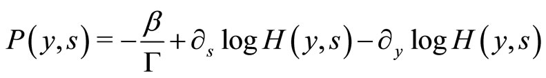 (20)
(20)
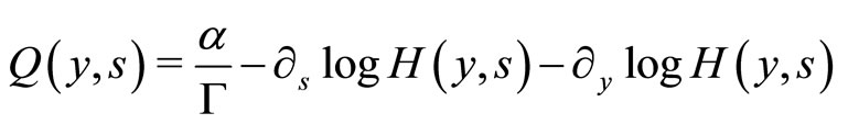 (21)
(21)
which actually reduces Equation (19) into the Telegraphist equation:
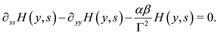 (22)
(22)
Accordingly, the dynamics given by Equation (8) with constant parameters can be exactly solved for any initial conditions  and
and . According to [42], the general solution reads as:
 (23)
(23)
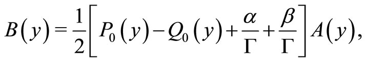
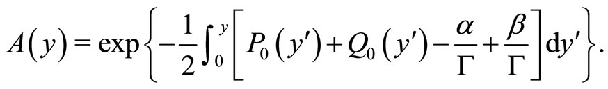
where  and where we have the following definitions:
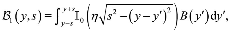
and

with  and
and  being the modified Bessel’s functions and:
 (24)
(24)
 (25)
(25)
Behavior of the Solutions
Though fully explicit and exact, the solution given by Equations (20) and (21) deserves discussion and interpretation for specific situations and this is precisely the objective of this section. In what follows, we will systematically choose  and unit velocities
 .
.
Let us here focus on the Bass’ dynamics that results when . This directly implies that
  and hence Equation (22) coincides with the ordinary wave equation. By definition of Bessel’s functions [46], we have that
  and
and , thus leading to the usual wave solution in the form:
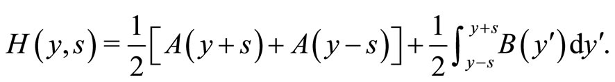 (26)
(26)
Due to the fact that , we expect that the agents’ population
  with velocity
  increases by opposition to the population
  of agents with velocity
  which is doomed to extinction. Let us now explore the transient nature of the solution and this for three types of initial conditions.
a) Initial conditions:  and
and 
In this case, the time-dependent solution reads as:
 (27)
(27)
as it can be checked directly from Equations (20) and (21). Equation (27) is clearly consistent with the fact that  and hence that no transitions from
  to
to  velocities occur. Hence, starting with all agents with velocity
 , they stay with their original velocity and the density
  is a uniformly traveling Dirac mass with velocity
  towards the positive
  -axis.
b) Initial conditions:  and
and 
Either by direct substitution into Equation (19) or alternatively by using Equations (20) and (21), one can verify that the time-dependent solution in this case reads as:
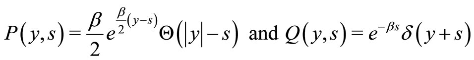 (28)
(28)
where  is a Heaviside cutoff function which identically vanishes for negative arguments. The dynamics
  of the spatial dispersion of the agents with velocity
  is illustrated in Figure 1.
The behavior of the solution given by Equation (28) can be easily understood. Indeed, the Dirac mass for  expresses the fact that agents with velocity
  are gradually depopulated at the rate
  for the benefit of agents traveling with velocity
  and hence migrating to
 . The Heaviside function
  expresses the fact that no agent can possibly be found at a distance larger than
  at time t (remember that the velocities here are
 ). It is worth observing that in the original Bass’ model, the adoption rate
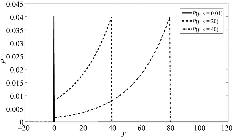
Figure 1. Spatial dispersion P(y, s) of the agents with velocity V+ = +1 for different times s = [0.01; 20; 40]. The initial conditions are given by P0(y) = 0 and Q0(y) = δ(y), α = 0 and β = 0.1. In this case, the agents are immediately segregated and there are no imitation processes.
given in Equation (16) is equal to . This overcomes the
  adoption rate that we will obtain below in Equation (29), due to the fact that in the present configuration, imitation process does not enter into play in our spatial model, which drastically moderates the overall adoption rate. Indeed, in this limiting regime the agents’ populations
  and
and  are immediately and definitively segregated, which hence never allows imitation processes to take effect (the unit rate discrepancy between the
  adoption rate occurring in Equation (16) and the
  rate in Equation (29) is obtained from the
  choice). The resulting temporal evolution of the agents’ overall adoption rate obtained in the present case (
 ), compared with the one of the original Bass’ model, will be illustrated later in Figure 4.
Finally, let us observe that, from Equation (28), one immediately obtains:
 (29)
(29)
thus showing that Equation (10) is fulfilled. In addition, for asymptotic times , Equation (29) indicates that all agents ultimately adopt the
  velocity as it is expected for the
  regime.
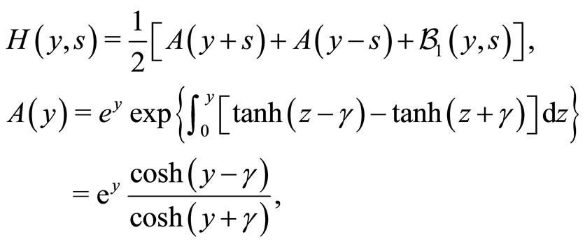
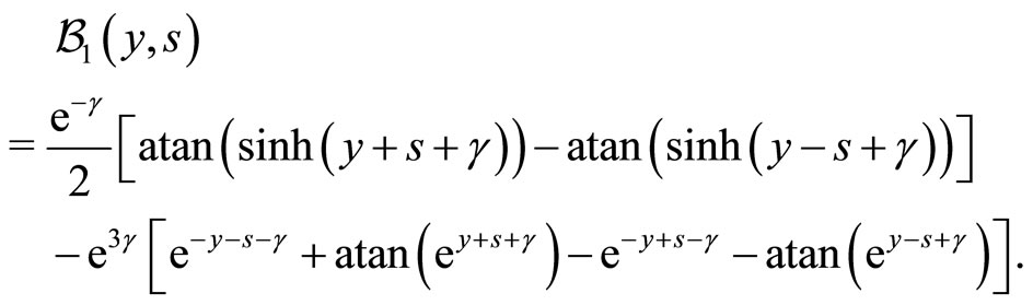
c) Initial conditions:
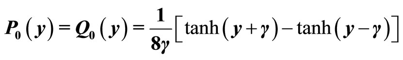
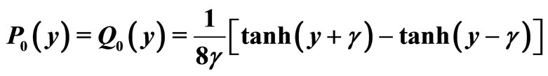
For these initial conditions and for the particular choice  and
and , the resulting time-dependent solution of our spatial Bass’ model is given by:
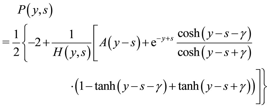 (30)
(30)
and
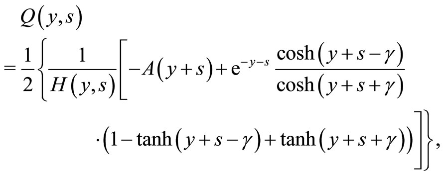 (31)
(31)
where
The spatio-temporal dynamics  of the agents with velocity
  is illustrated in Figure 2. The joint evolutions of
  and
and  (representing agents with velocity
  and
and  respectively) are drawn in Figure 3.
In the present configuration, the two types of agents have an identical initial spatial distribution (i.e.
 ). Hence, half of the agents have initially the velocity
 , the other half having the velocity
 , i.e.
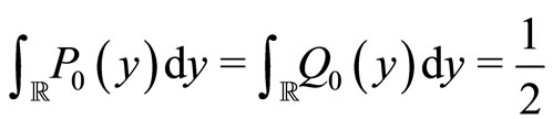 .
.
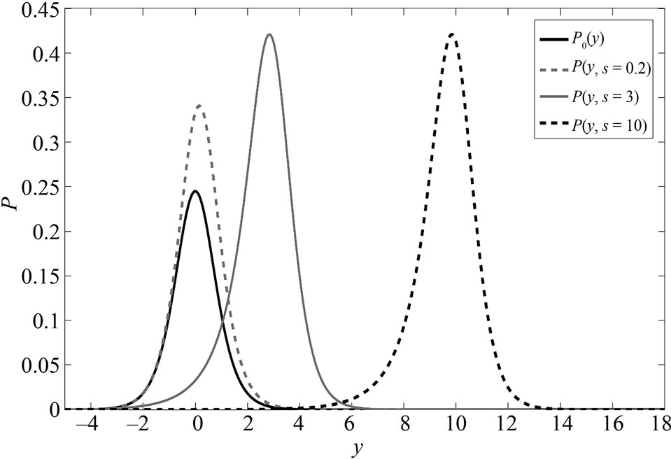
Figure 2. Spatial dispersion P(y, s) of the agents with velocity V+ = +1 for different times s = [0; 0.2; 3; 10]. The initial conditions are given by
 ,
,
 ,
,  and
and .
.
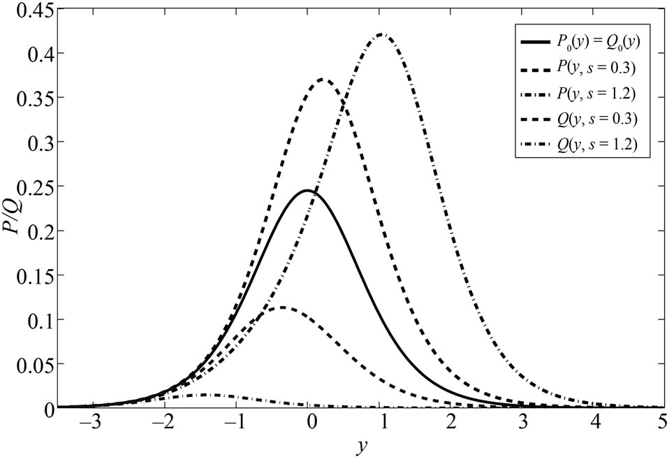
Figure 3. Spatial dispersions P(y, s) and Q(y, s) of the agents with velocity V+ = +1 and V– = –1 respectively, for times s = [0; 0.3; 1.2]. The initial conditions are given by
 ,
,
 ,
,  and
and .
.
The spatio-temporal behavior of the solution given by Equations (30) and (31) can be split into two different time phases. For short times of the dynamics, the overlap between  and
and  is non-null (i.e. the two populations of agents
  and
and  are not spatially segregated), thus leading to strong imitation processes between the agents. Agents are changing their velocity from
  to
to  due to both imitation and spontaneous transitions. Accordingly,
  is gradually depopulated for the benefit of
 . The imitation processes are decreasing as the overlap between
  and
and  gets smaller, but the rate
  of spontaneous transitions from
  to
to  remains itself constant with time. In the time asymptotic regime, almost all the agents have adopted velocity
 , leading
  to behave as a probability density uniformly traveling with velocity
  towards the positive
  -axis.
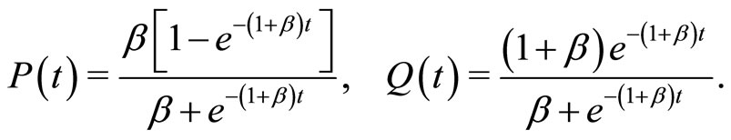
In Figure 4, the temporal evolution of the overall adoption rate  of the agents is illustrated and compared to the one observed for the Bass’ original model. For the present configuration, the overall adoption rate stands between
 , the rate observed for our spatial Bass’ model in absence of imitation processes (Section 3.1.b), and
  the rate obtained for the original aggregated Bass’ model. Hence, in general, the overall adoption rate of our spatial Bass’ model will be equal to
 with
with  depending on the initial distributions of the agents and on the model parameters. Remember that the imitation rate (and hence the overall adoption rate) is controlled by the number of neighbors that each agent effectively observes during the imitation process. In the aggregated (original) Bass’ model, this number is maximum as each agent systematically observes
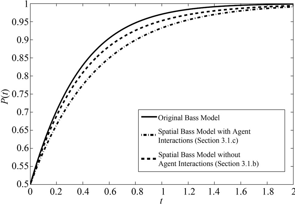
Figure 4. Temporal evolution of the overall adoption rate P(t): 1) for the original Bass’ model, 2) for our spatial Bass’ model when there are imitation processes (Section 3.1.c) and 3) for our spatial Bass’ model when there are no imitation processes because the two populations of agents  and
and  are immediately segregated (Section 3.1.b).
the global population of agents. In the limiting regime of Section 3.1.b, the number of observed agents is equal to 0 as the two populations of agents  and
and  are initially and hence permanently segregated, thus allowing no imitation processes.
4. Conclusions and Perspectives
Often, agents’ remoteness may naturally reduce the efficiency of imitation processes, a feature that is totally absent in the original aggregated Bass’ approach. Incorporating a spatial dimension into the Bass’ dynamics is however not a minor extension. It transforms indeed a nonlinear single dimension dynamics into a nonlinear infinite dimensional field dynamics for which, in general, no solution methods are available. It is hence remarkable that our spatial generalization of the original Bass’ dynamics leads to a class of models for which the evolution of the resulting spatio-temporal patterns can be exactly calculated. Indeed, the quadratic nonlinearity, due here to the underlying imitation mechanism, coincides with the collision term found in a solvable Boltzmann equation, the RW dynamics, used for gas models in mathematical physics. Our paper points out that the RW dynamics, solvable via a linearizing logarithmic transformation, offers a unique, synthetic and exact modeling framework to study nonlinear features generated by spatio-temporal imitation processes in economics systems.
In this paper, we mainly focused on Bass’ dynamics which does not allow back transitions (i.e. , implying no transitions from
  to
to ). Allowing
 , regimes involving shock waves with propagating velocities w emerge and the velocity range is
 [42]. When a dominant spontaneous tendency to stay in the
  state exists (i.e.
 ), imitations enhance the spontaneous
  -flow from
  and may lead to a time-independent (i.e.
 ), shock type inhomogeneous solution. Depending on the initial conditions, this marginal stationary
  solution separates two regimes of shocks propagating with either positive or negative velocities, a rich dynamical behavior that deserves further investigations in economy.
REFERENCES
- E. Mansfield, “Technical Change and the Rate of Imitation,” Econometrica, Vol. 29, No. 4, 1961, pp. 741-766. doi:10.2307/1911817
- Z. V. Griliches, “Hybrid Corn: An Exploration in the Economics of Technological Change,” Econometrica, Vol. 25, No. 4, 1957, pp. 501-522. doi:10.2307/1905380
- Z. V. Griliches, “Hybrid Corn and the Economics of Innovation,” Science, Vol. 132, No. 3422, 1960, pp. 275- 280. doi:10.1126/science.132.3422.275
- F. Bass, “A New Product Growth Model for Consumer Durables,” Management Science, Vol. 15, No. 5, 1969, pp. 215-227. doi:10.1287/mnsc.15.5.215
- J. A. Schumpeter, “Business Cycles: A Theoretical, Historical and Statistical Analysis of the Capitalist Process,” McGraw-Hill, New York, 1939.
- B. Jovanovic and R. Rob, “Long Waves and Short Waves: Growth through Intensive and Extensive Search,” Econometrica, Vol. 58, No. 6, 1990, pp. 1391-1409. doi:10.2307/2938321
- R. Pastor-Satorras and A. Vespigniani, “Epidemic Spreading in Scale-Free Networks,” Physics Review Letters, Vol. 86, No. 14, 2001, pp. 3200-3203. doi:10.1103/PhysRevLett.86.3200
- E. Glaeser, B. Sacerdote and J. Scheinkman, “Crime and Social Interactions,” Quarterly Journal of Economics, Vol. 111, No. 2, 1996, pp. 507-548. doi:10.2307/2946686
- R. Cont and J. P. Bouchard, “Herd Behavior and Aggregate Fluctuations in Financial Market,” Macroeconomic Dynamics, Vol. 4, No. 2, 2000, pp. 170-196. doi:10.1017/S1365100500015029
- A. Corcos, J.-P. Eckmann, A. Malaspinas, Y. Malevergne and D. Sornette, “Imitation and Contrarian Behavior: Hyperbolic Bubbles, Crashes and Chaos,” Quantitative Finance, Vol. 2, No. 4, 2002, pp. 264-281. doi:10.1088/1469-7688/2/4/303
- P. Dai Pra, W. J. Runggaldier, E. Sartori and M. Tolotti, “Large Portfolio Losses: A Dynamic Contagion Model,” Annals of Applied Probability, Vol. 19, No. 1, 2009, pp. 347-394. doi:10.1214/08-AAP544
- U. Horst, “Stochastic Cascades, Credit Contagion and Large Porfolio Losses,” Journal of Economic Behavior & Organization, Vol. 63, No. 1, 2007, pp. 25-54. doi:10.1016/j.jebo.2005.02.005
- D. Lopez-Pintado and D. J. Watts, “Social Influence, Binary Decisions and Collective Dynamics,” Rationality and Society, Vol. 20, No. 4, 2008, pp. 399-443. doi:10.1177/1043463108096787
- D. Lopez-Pintado, “Diffusion in Complex Social Networks,” Games and Economic Behavior, Vol. 62, No. 2, 2008, pp. 573-590. doi:10.1016/j.geb.2007.08.001
- F. Collet, P. Dai Pra and E. Sartori, “A Simple MeanField Model for Social Interactions: Dynamics, Fluctuations, Criticality,” Journal of Statistical Physics, Vol. 139, 2010, pp. 820-858. doi:10.1007/s10955-010-9964-1
- T. W. Valente, “Network Models of Diffusion of Innovations,” Hampton Press, New York, 1995.
- W. Brock and S. N. Durlauf, “Discrete Choice with Social Interactions,” Review of Economic Studies, Vol. 68, No. 2, 2001, pp. 235-260. doi:10.1111/1467-937X.00168
- L. Blume, “The Statistical Mechanics of Strategic Interactions,” Games and Economic Theory, Vol. 5, 1993, pp. 387-424. doi:10.1006/game.1993.1023
- M. Schultz, “Statistical Physics and Economics—Concepts, Tools and Applications,” Springer Verlag, Berlin, 2003.
- L. Blume and S. N. Durlauf, “The Interactions-Based Approach to Socioeconomic Behavior,” Mimeo, Department of Economics, University of Wisconsin, 1998.
- W. Brock and S. N. Durlauf, “Interaction-Based Model,” In: J. Heckmann and E. Leamer, Eds., Handbook of Econometrics, Vol. 5, North Holland, 2001, pp. 3297- 3380.
- G. Ellison, “Learning, Local Interactions and Coordination,” Econometrica, Vol. 61, No. 5, 1993, pp. 1047-1071. doi:10.2307/2951493
- G. Ellison and D. Fudenberg, “Rules of Thumb for Social Learning,” Journal of Political Economy, Vol. 101, 1993, pp. 612-644. doi:10.1086/261890
- R. Andergassen, F. Nardini and M. Ricottilli, “Innovation Waves, Self-Organized Criticality and Technological Convergence,” Journal of Economic Behavior & Organization, Vol. 61, No. 4, 2006, pp. 710-728. doi:10.1016/j.jebo.2004.07.009
- D. Levine, “Is Behavioral Economics Doomed?” Max Weber Lecture, 2009.
- D. Levine and D. Fudenberg, “Learning and Equilibrium,” Annual Review of Economics, Vol. 1, No. 1, 2008, pp. 385-419.
- D. Levine and W. Pesendorfer, “Evolution of Cooperation through Imitation,” Games and Economic Behavior, Vol. 58, No. 2, 2007, pp. 293-315. doi:10.1016/j.geb.2006.03.007
- U. Horst, “Dynamic Systems of Social Interactions,” Journal of Economic Behavior & Organization, Vol. 73, No. 3, 2010, pp. 158-170. doi:10.1016/j.jebo.2009.09.007
- A. Foster and M. Rosenzweig, “Learning by Doing and Learning from Others: Human Capital and Technical Change in Agriculture,” Journal of Political Economy, Vol. 103, No. 6, 1995, pp. 1176-1209. doi:10.1086/601447
- E. M. Rogers, “Diffusion of Innovations,” Free Press, New York, 1992.
- P. Krugman, “Geography and Trade,” MIT Press, Cambridge, 1991.
- M. P. Feldman, “Knowledge Complementary and Innovation,” Small Business Economics, Vol. 6, 1994, pp. 363-372. doi:10.1007/BF01065139
- M. P. Feldman, “The Geography of Innovation,” Kluwer Academic Publishers, Boston, 1994.
- A. C. Case, “Spatial Patterns in Household Demand,” Econometrica, Vol. 59, No. 4, 1991, pp. 953-965. doi:10.2307/2938168
- D. B. Audretsch and M. P. Feldman, “Knowledge Spillovers and the Geography of Innovation and Production,” American Economic Review, Vol. 86, No. 3, 1966, pp. 630-640.
- Z. J. Acs, D. B. Audretsch and M. P. Feldman, “Real Effects of Academic Research: Comment,” American Economic Review, Vol. 82, No. 1, 1992, pp. 363-367.
- Z. J. Acs, D. B. Audretsch and M. P. Feldman, “R & D Spillovers and Recipient Firm Size,” Review of Economics and Statistics, Vol. 76, No. 2, 1994, pp. 336-340. doi:10.2307/2109888
- A. Jaffe, M. Trajtenberg and R. Henderson, “Geographic Localisation of Knowledge Spillovers as Evidenced by Patent Citations,” Quarterly Journal of Economics, Vol. 108, No. 3, 1993, pp. 577-598. doi:10.2307/2118401
- G. A. Akerlof, “Social Distance and Social Decisions,” Econometrica, Vol. 65, No. 5, 1997, pp. 1005-1027. doi:10.2307/2171877
- T. Vicsek, A. Czirok, E. Ben-Jacob, I. Cohen and O. Shochet, “Novel Type of Phase Transition in a System of Self-Driven Particles,” Physical Review Letters, Vol. 75, No. 6, 1995, pp. 1226-1229. doi:10.1103/PhysRevLett.75.1226
- F. Cucker and S. Smale, “Emergent Behavior in Flocks,” IEEE Transactions on Automatic Control, Vol. 52, No. 5, 2007, pp. 852-862. doi:10.1109/TAC.2007.895842
- T. W. Ruikgrok and T. T. Wu, “A Completely Solvable Model of the Nonlinear Boltzmann Equation,” Physica A, Vol. 113, No. 2, 1982, pp. 401-416. doi:10.1016/0378-4371(82)90147-9
- M.-O. Hongler, O. Gallay, M. Hülsmann, P. Cordes and R. Colmorn, “Centralized Versus Decentralized Control —A Solvable Stylized Model in Transportation,” Physica A, Vol. 389, No. 19, 2010, pp. 4162-4171. doi:10.1016/j.physa.2010.05.047
- M.-O. Hongler and L. Streit, “A Probabilistic Connection between the Burgers and a Discrete Boltzmann Equation,” Europhysics Letters, Vol. 12, 1990, pp. 193-197.
- E. Gutkin and M. Kac, “Propagation of Chaos and the Burgers’ Equation,” SIAM Journal of Applied Mathematics, Vol. 434, No. 4, 1963, pp. 971-980.
- M. Abramowitz and I. Stegun, “Handbook of Mathematical Functions,” Dover, see entry 9.6.