Journal of Mathematical Finance
Vol. 3 No. 2A (2013) , Article ID: 30542 , 10 pages DOI:10.4236/jmf.2013.32A001
Investment Reluctance in Supply Chains: An Agent-Based Real Options Approach
1Leibniz Institute of Agricultural Development in Central and Eastern Europe (IAMO), Halle, Germany
2Department for Agricultural Economics and Rural Development, Faculty of Agricultural Sciences, University of Goettingen, Göttingen, Germany
Email: balmann@iamo.de, kataria@iamo.de, oliver.musshoff@agr.uni-goettingen.de
Copyright © 2013 Alfons Balmann et al. This is an open access article distributed under the Creative Commons Attribution License, which permits unrestricted use, distribution, and reproduction in any medium, provided the original work is properly cited.
Received February 5, 2013; revised March 17, 2013; accepted March 28, 2013
Keywords: real options; supply chain; agent-based models; genetic algorithms
ABSTRACT
This paper shows how agent-based stochastic approaches can provide a complementary and more flexible approach to study investment incentives and price dynamics in a real options framework. We particularly study the case of twostage production chains in which one sector produces an intermediate product and the other the final product, and the intermediate product is traded on the spot market. An agent-based competitive model using a genetic algorithm allows us to explicitly model the behaviors and interactions of the firms competing in each subsector and trading the intermediate product with each other on a spot market, and optimal investment strategies can be identified.
1. Introduction
According to the real options approach, irreversible investment decisions under uncertainty should consider the opportunity costs of deferring the investment decision in order to obtain improved information on the involved risks ([1,2]). Particularly [3,4] illustrate how option values as well as optimal investment triggers can be determined. Numerous empirical applications apply the developed concepts and show that price uncertainty creates investment reluctance beyond risk aversion. The very most of these studies ignore strategic aspects and presume the uncertainty to be exogenous. This simplification can be justified by [5] who showed that under perfect competition the endogenous price response to demand shocks leads to price dynamics with identical investment triggers, i.e. a myopic investor can ignore competition. Comparatively little research has been undertaken to study the more complex strategic interactions. Nevertheless, there are a number of analyses which identify equilibrium conditions for game theoretic settings, including [6-8]. A particular strength of these studies is that the equilibrium conditions are based on closed-form analytical solutions. While this allows the derivation of quite general results, also limitations exist such as restrictive assumptions regarding e.g. the assumed stochastic process and homogeneity.
Because of the limitations of the analytical approaches, the objective of this paper is to illustrate that agent-based stochastic approaches may provide a complementary approach to study more flexible settings. Therefore, we show how agent-based models can be applied to a real options framework and what additional insights into the resulting market dynamics they can provide. Starting point is a simple two-stage value chain in which one sector produces an intermediate product while a second sector produces the final product. An empirical application of such a situation is provided by [9] who study the pork chain in Finland using a real options approach. The pork chain also provides a good example for our setting as we can presume a polypolistic market structure, a one to one relation between the two sectors as well as a nonstorable intermediate product. This results in a high volatility of the intermediate product’s price. To compare the alternative production chains, we apply an agent-based framework. As an example of a perfectly integrated system, every firm can invest in an integrated system in which the intermediate product and the final product are produced in equal amounts. In the alternative production system, one group of firms can invest in the intermediate product, while a second group of firms can invest in the final product. The intermediate product is assumed to be traded on a spot market. As source of uncertainty, it is assumed that an iso-elastic demand curve for the final product follows a random walk.
Within this setting, the subsectors and the spot market interaction are explicitly modeled. Instead of looking at the market at an aggregate level, we develop an agentbased model which follows a bottom-up approach by explicitly modeling the firms and their behavior, as well as their interaction. In this discrete-time model, a number of agents represent identical firms which compete within their subsector and trade with another subsector. The firms identify optimal investment strategies for Monte Carlo simulations of demand shocks for the final product and can invest irreversibly into production assets without knowing how the market environment will evolve in the future. Producers of the intermediate product and producers of the final product are assumed to be aware of the investment strategies and the production capacities of other producers, i.e. we presume a rational expectation hypothesis. Moreover, the producers of the intermediate product are assumed to know the actually existing production capacity of the producers of the final product, but not the actual (dis-)investments. Every firm invests according to its individual investment trigger which is derived by linking Monte Carlo simulations of the agentbased model with a genetic algorithm (cf. [10,11]). The combination with genetic algorithms allows identifying dynamic investment equilibria for polypolistic as well as for oligopolistic settings by either using a social or an individual learning approach ([12]). As we address a polypolistic market structure, we apply a social learning approach.
The model is adapted to parameters and cost structures reflecting pork production in the EU and thus considers, as in [9], piglets as the intermediate product and finished hogs as the final product. Our analysis shows that the closed system and spot market solutions both lead to very similar production dynamics. Differences in investment behavior are only marginal, even in the case of inelastic demand respectively high price flexibility for the intermediate product. This contradicts what [9] found for pork production chains in Finland but the differences can be attributed to the different methodological approaches applied; e.g. we here model firms’ behaviors explicitly assuming rational expectations instead of looking at the market at an aggregate level.
The outline of this paper is the following. First, the model and the application of the genetic algorithm are described, followed by a description of the parameters reflecting the pork supply chain which are used in the simulations. The model is thereafter validated and the simulation results presented. Summary and conclusions end the paper.
2. Model and Scenarios
2.1. An Agent-Based Investment Model of a Two Stage-Value Chain
In order to model the interactions between firms within a two-stage value chain in which one sector produces an intermediate product and the other sector produces the final product, an agent based approach is used. This allows for explicitly modeling the behaviors and interactions of the firms competing in each subsector and trading the intermediate product with each other on a spot market. The two-stage scenario is compared with a scenario of one sector producing the final product in a onestage production system, i.e. a vertically integrated (or closed) production system. We begin the model description by presenting the investment problem in the latter case, which is similar to [11,13]. Thereafter we extend the model to the case of a two-stage system in which the intermediate and final products are produced by the separate sectors and traded on a spot market.
In a time-discrete setting it is assumed that N firms repeatedly have the opportunity to invest in identical assets or a fraction thereof, and that no firm has initially invested. The asset stock of firm n has a maximum size of 1 and can be used by the firm to produce up to  units of output per period. Size, investment outlay and production are assumed to be proportional, i.e. there are no economies of scale. If a firm invests for the first time, its maximum initial investment outlay
  is
is . The investment outlay
  is assumed to be totally sunk after the investment is carried out. In every future period, a geometrical decay of the asset with a depreciation rate
  is assumed. However, in every period, the firms can invest or reinvest in order to increase production or to regain a production capacity of up to one unit of output. The total asset of firm
  in period
  can thus be written as:
 (1)
(1)
such that  and where
  is the additional available asset in
  due to investment decision in t.
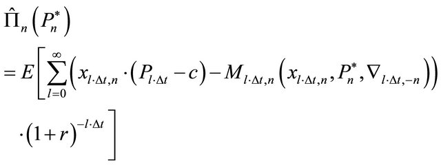
Each firm’s investment decisions aim to maximize the expected net present value of future cash flows by choosing an optimal investment trigger, . The objective function of firm
  is thus represented by:
 (2)
(2)
 (3)
(3)
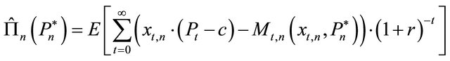
and where is the output price in period t, c is the variable production costs per unit of output and period, and r is the risk-free interest rate. To capture competition, the firms and their interaction are represented in an agentbased setting in which the firms are represented as agents that perceive their environment and respond to it individually and autonomously ([14]).
The environment of a firm n consists of two parts: the behavior of other firms and the demand for outputs. Total supply in period t is
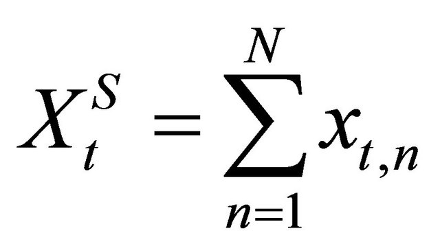 (4)
(4)
and demand is
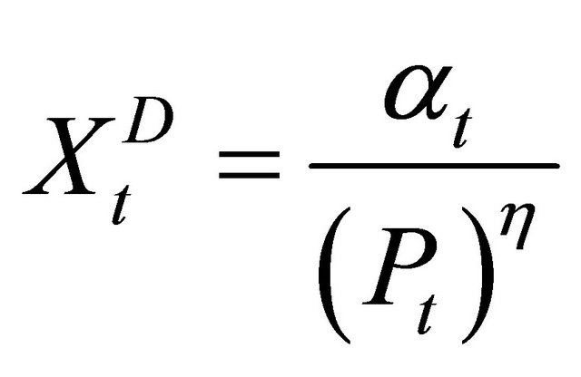 (5)
(5)
where  is the elasticity of demand. For the identity of demand and supply, (6) must hold:
 (6)
(6)
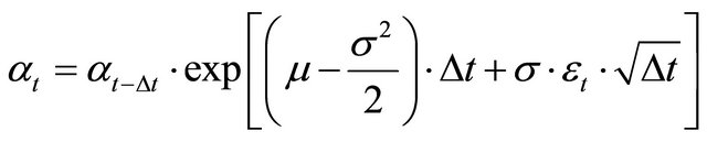
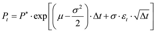
The demand parameter  is assumed to follow a geometric Brownian motion. Assuming discrete time, this can be modeled as
 (7)
(7)
with a volatility , a drift rate μ, and where εt is a normally distributed random number and ∆t is the time step length.
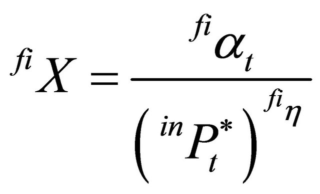
Firm n invests in period t if the expected price  is larger than or equal to the trigger price
 . For the expected price
 , the following holds:
 with (8)
 and (9)
The questions now are: Which firms invest and how much do they invest? It is assumed that firms with lower trigger prices have a stronger tendency to invest. Consequently, all firms can be sorted according to their trigger prices, starting with the lowest investment trigger, i.e.,
 . It is considered that: 1) If firm n does not invest in
 , firm
  will also not invest in t, i.e.,
  , 2) If firm n does invest in t, then firm
  will invest
  in t, i.e.
  , 3) In every period
 , a marginal (or last) firm
  exists which invests
  such that the expected price for the next period is equal to the investment trigger of firm
 , i.e.
  with
with  and
and  1.
1.
The investment of firm  can be computed according to
 (9)
(9)
 (10)
(10)
 (11)
(11)
 can now be identified by iteratively testing all firms for
 . The last firm with a positive investment is
 .
.
Equation (11) is an equilibrium condition: All firms which fully invest and hence produce at maximum capacity have trigger prices which are less than or equal to the trigger price of firm  which is also equal to the expected price for t + ∆t. All firms which do not invest have trigger prices which are higher than or equal to the expected price for t + ∆t.
For a given set of trigger prices,  , and arbitrary initializations of
 , the expected profitability of each strategy
 (12)
(12)
can be simultaneously determined by a sufficiently high number of repeated stochastic simulations of the market. Due to the competitive environment and identical production technologies, the expected profitability of a rational strategy will fulfill the zero-profit condition given all other strategies are also rational.
Until now, the model reflects a firm’s investment problem for a closed production system in which the intermediate product and the final product are produced in appropriate amounts within a production unit. The investment cost I is then assumed to cover the costs for both production assets, i.e.,  , where the italic superscripts on the left side denote intermediate and the final product respectively.
The question is now what the consequences of a spot market relationship between the producers of the intermediate and final product for their investment triggers are. In such a system, the production capacity of the producer of the final product can be interpreted as a demand parameter of the producers of the intermediate product, i.e.
 (13)
(13)
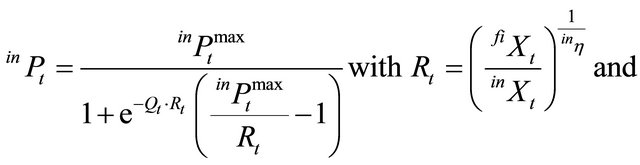
Regarding the price formation for the intermediate product, a logistic relationship is considered. This allows for a maximum price of  to avoid that the expected gross margin of the final product is negative as well as to ensure that there is a minimum price for the intermediate product
 , assuring non-negativity of gross margins for the intermediate product. Considering isoelastic demand for the intermediate product, then the market equilibrium for the first-stage producers fulfills
 (14)
(14)
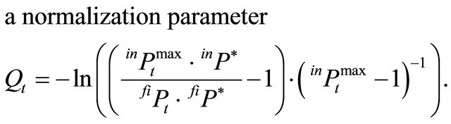
The normalization parameter  ensures that in case of identity of production capacities of the two producers, the price of the intermediate product is proportional to the relation of the price triggers of the final and intermediate products. Rt is to be interpreted as a price response coefficient considering the relation of supply and demand for the intermediate product where
  represents a kind of “demand elasticity” for the intermediate product.
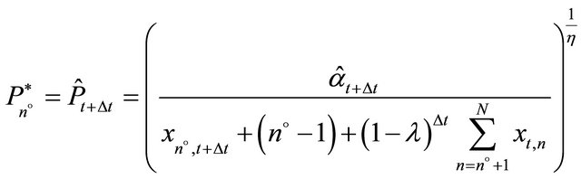
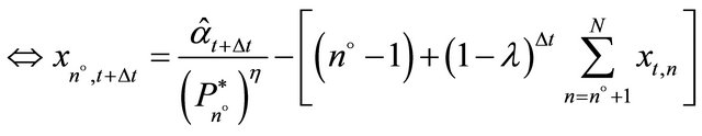
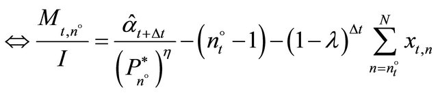
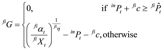
The intermediate producer n invests if the expected price for the intermediate product  is larger than or equal to her trigger price
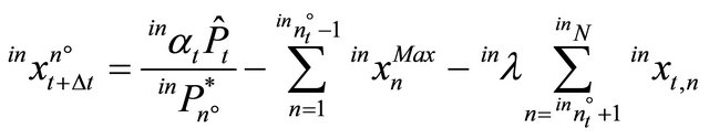
 . Total production of the intermediate product in the period t + Δt is
  where
where  is the price trigger of the marginal investor, n˚. The production of the intermediate product by the marginal investor in the period t + Δt is
 (15)
(15)
where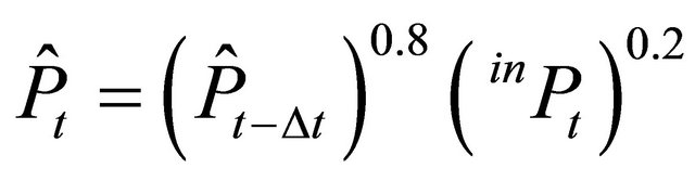 , i.e. an adaptive price expectation is used as a proxy2. Note that in contrast to the one-stage case, the net return for the producers of the final products
  must be adjusted by the price of the intermediate product and other variable costs in the second stage,
 . Additionally, since the second stage producers would not spend more money on the intermediate product and other variable costs than the expected return for the final product, the expected minimum net return is zero which is formalized in equation (16):
 (16)
(16)
The following is assumed to hold for the second stage producers:
 (17)
(17)
As for the closed system, the optimal trigger prices,  and
and , are determined by combining the multifirm market models with a genetic algorithm (GA), which is described in the following section.
2.2. The Genetic Algorithm and Its Implementation
Even though many variations of GA exist, some common elements can be recognized (cf. [15-18]). The first task of a GA application is to specify a way of representing each possible solution or strategy as a string of genes located on one or more chromosomes. Since our problem is relatively simple, i.e. we are searching for a single value (every strategy consists just of a certain trigger price) and we can assume a convex search space, we take the investment trigger as a real value and apply the GA operators to the nominal value of trigger price. The second task is to define a population of genomes to which the genetic operators, i.e. selection, crossover and mutation, can be applied. The population size is set equal to , the number of firms. This allows the direct mapping of the set of genomes to the various firms’ strategies, i.e., every firm’s trigger price in our model is represented by one genome from the genome population.
After random initialization, the genome population passes, in every generation, through the steps of fitness evaluation, selection, recombination (crossover) and mutation. These operators are in our model implemented in the following way:
Fitness evaluation: The fitness value is directly derived from the strategy’s average profitability for 1000 to 5000 repeated stochastic simulations of the market model.
Selection: The selection procedure replaces the least profitable strategies with the most profitable ones. The higher the relative profitability, the higher is the probability for replication.
Recombination: For recombination or crossover, the geometric average of two parent genomes is calculated resulting in one offspring which replaces one parent.
Mutation: Mutation is implemented here by multiplying every solution by chance (with a small likelihood) with a random number within a closed range (e.g., [0.95, 1.05]. The mutation likelihood, as well as the range of the random number, may be chosen according to experience or according to the already obtained results.
These steps are repeated until the model converges (i.e. the strategies are similar from one generation to the other). A flow diagram of this procedure can be found in Figure A1 in the appendix. In one particular point, our GA application deviates from the conventional use of GA for optimization problems. Here, the GA is not just used to solve a complex optimization problem in which the goodness of the solution respectively the problem at hand are directly related. In our case, the goodness of a solution rather depends on the alternative solutions generated by the GA, i.e., the genomes compete directly. Thus, we are applying the GA to a market and we are searching not just for an optimal solution, but for an equilibrium solution (i.e., the Nash-equilibrium strategy). A number of publications during the past 15 years show that agentbased GA approaches function quite well for analyzing such strategic interactions. Examples and discussions are given, for instance in [10,19-22]. However, as [12] shows, one has to differentiate whether one aims to identify an equilibrium for perfect competition or for oligopolistic competition. Since we assume perfect competition, in our model all agents on each production level (i.e., integrated firms, intermediate product firms, final product firms) share the same genome population. We thus apply the concept of social learning [12]. Nevertheless, for the spot market model, the genome populations for investment triggers on the intermediate and the final product stage co-evolve, i.e., optimal triggers on the intermediate and the final stage depend on each other.
2.3. Applying the Model to the Pork Production Chain
The model described above is applied to the pork production chain, in which piglets represents the intermediate product used in the finishing (hog) stage. There is a one to one relation between the two sectors making this a particularly suitable example for our model. The calculations are based on an interest rate of r = 6%, a depreciation rate of 5% (in the base scenario), and a time step length of 0.25. This implies that an investment cost of  implies a periodical fixed production cost of 1 per unit of output. For modeling external markets shocks through demand shocks a drift rate, μ, is assumed to be zero and the volatility, σ, is assumed to be either 5%, 10% or 15%. The total time span T simulated in every stochastic simulation is determined as 100 years. For later periods, the expected returns are set equal to the returns in year 100. The possible error can be assumed to be negligible since later returns are discounted by more than 99.7%.
Regarding production costs, it is assumed that the total production cost per piglet is 2.5 (which, multiplied by 20, corresponds to 50 EUR per piglet), of which 1.0 (20 EUR) is fixed costs (related to the annual irreversible investment cost) and 1.5 (30 EUR) is variable costs. The production costs for pork (per hog) are 3.5 (which multiplied by 20, corresponds to 70 EUR per hog), of which 1.0 (20 EUR) is fixed costs (related to the annual irreversible investment cost) and 2.5 (50 EUR) is variable costs, plus the cost of the piglet. These production costs correspond approximately to the cost structure of pig production within the EU3.
3. Validation and Results
3.1. Validation of the Model
In order to validate the agent-based model of multiple competing farms, it can be shown that the agent-based approach leads for the standard case of a one-stage production system to the same dynamics as a direct simulation of the price dynamics.
Consider the existence of an equilibrium investment trigger  at which all firms invest and assume that in period
  firms have invested according to
 . From equations (6) and (7) we know that after the investment decisions are made,
  purely depends on the relation of
  and
and . Hence, the price in t will be
 . (18)
Consider now that the actual price in period t is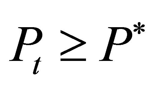 . Then the firms will respond and invest such that
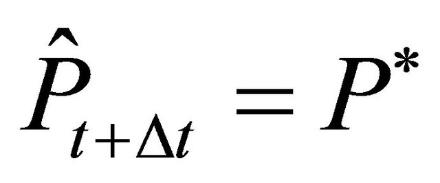 . For
. For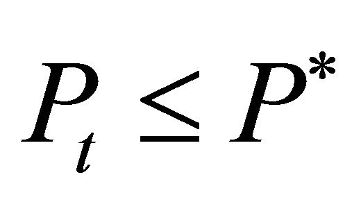 , two cases have to be differentiated. If
 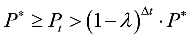 then some firms will reinvest, such that
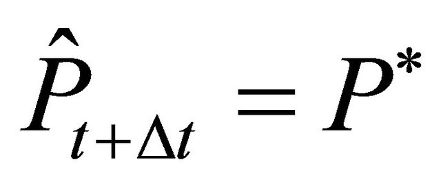 . Otherwise, if
 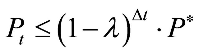 no firm will reinvest and
 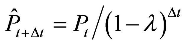 . With this knowledge and in accordance with equations (1) to (12) the price dynamics can be described as:
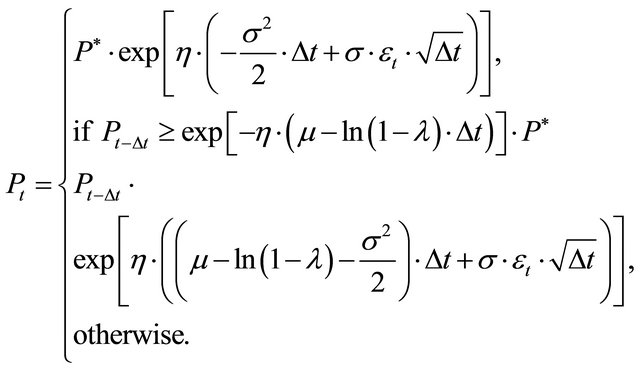 (19)
(19)
Equation (19) represents the discrete time version of a so-called regulated Brownian motion, which permits the simulation of price dynamics directly, i.e., without the explicit representation of firms ([5,25]). Moreover, (19) can be used to determine the equilibrium investment trigger . Repeated stochastic simulations of Equation (19) for various values of
  should reveal that the zeroprofit condition will only be fulfilled if
  is equal to the equilibrium investment trigger. If
  is higher, the dynamics should allow for profits. If
  is smaller, this should imply losses. Accordingly, the equilibrium trigger price
  can be determined by minimizing the square of the expected profits, i.e.
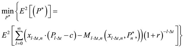 (20)
(20)
with 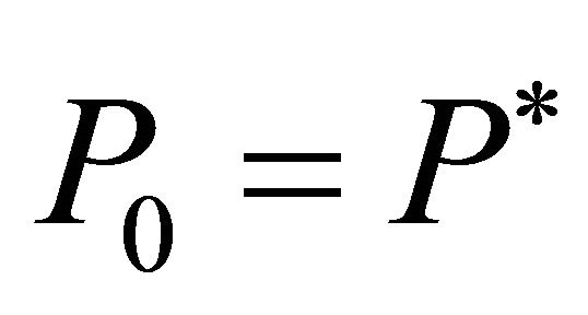 and Pt follows equation (19).
Figure 1 shows that for identical trigger prices,  , and identical αt, the agent-based model and the direct price simulation lead to an identical price path. Moreover, the direct price simulations lead to identical trigger prices. Hence, the direct price simulation validates the results of the agent-based approach.
3.2. Results
Our results suggest that vertical integration does not strongly influence production volume and welfare. This is shown by Figure 2. For given dynamics of demand for pork, the scenarios lead to very similar price paths. The fluctuations in piglet prices in the simulated data arise because we assume there is not an exact adjustment of piglet production to the hog finishing capacities (this is implied by equation (14)).
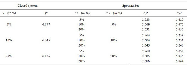
Table 1 presents the trigger prices for investments under alternative assumptions concerning the parameter values for demand elasticities and volatility. For a given demand elasticity, the trigger prices for pork in the closed
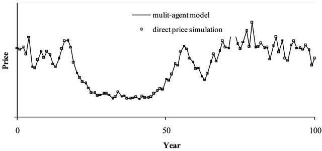
Figure 1. Price dynamics in the agent-based model and in the direct price simulation (identical trigger prices for all genomes).
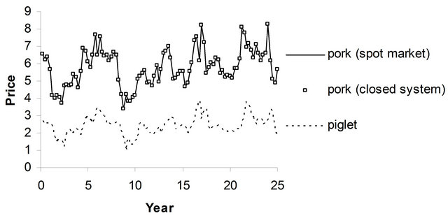
Figure 2. Price paths as results from alternative scenarios (identical trigger prices, P*, and demand parameters, αt, for pork assumed, 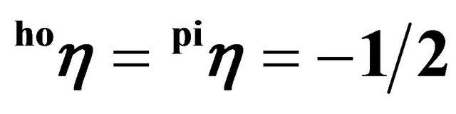
 , and
, and  ).
).
systems do not differ substantially from the trigger prices of the spot market solution. In general, the difference is below 0.1% of the trigger price respectively 0.5% of the difference between the trigger price and the total production cost4. Thus, our results suggest that from a pure real options perspective, a stronger vertical integration does not significantly increase investments. This result contradicts the empirically-based results of, e.g., [9]. This may be explained by our implicit assumption of rational expectations regarding the behavior of competitors as well as the information about the current production capacities on the other production stage. This, however, is not unrealistic considering that public statistics usually provides information about production capacities of piglet and pork producers. Moreover, capacity differences are usually reflected in market prices, which give signals to invest or disinvest in reasonable time. In the following analysis, the assumptions of σ = 10% and  will be used (estimated demand elasticities for pork that can be found in the literature are often around −0.55).
In order to analyze the impact of the price flexibility on the spot market for piglets, demand elasticities for piglets have been varied. In Table 2, it is illustrated that the trigger prices are not affected substantially when varying the demand elasticity for piglets. Accordingly, the above presented findings can be considered as robust against assumptions regarding the definition of the piglet prices.
A variation of the useful lifetime of the breeding barns (represented by the depreciation rate) changes the price dynamics for piglets. This is illustrated in Table 3. However, variations of the depreciation rate of breeding barns do not affect the trigger price for finishing barns strongly. Higher depreciation rates for piglet breeding barns lower their trigger price as a consequence of the higher flexibility of piglet production. Vice versa, lower depreciation
Table 1. Trigger prices in closed systems and spot market solutions for different demand elaticities .
.
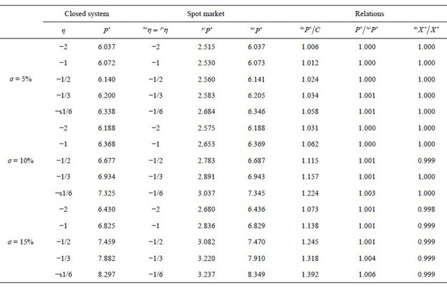
Table 2. Trigger prices in closed systems and spot market solutions for different demand elasticities for piglets (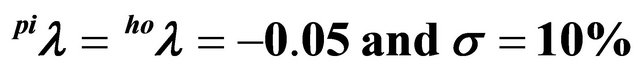
 ).
).

Table 3. Trigger prices depending on depreciation rates .
.
rates for piglet breeding barns lead to a higher volatility of the piglet prices and therefore to higher trigger prices.
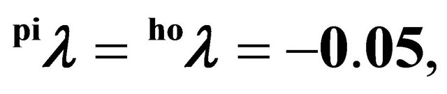
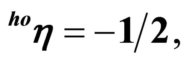
Figures 3 and 4 illustrate the dynamics of prices for hogs and piglets for different depreciation rates for breeding barns ( and
and  for
for  ). Note that if the depreciation rates for piglet and hog producers are equal, higher depreciation rates lead to lower trigger prices and vice versa. Higher depreciation is equivalent to higher flexibility of adjustment. That is to say, investments with high depreciation rates can be considered as less irreversible and thus also investment reluctance is lower. On the aggregate level, this means that production can relatively quickly respond to negative demand shocks. In [25] it is shown that the depreciation rate corresponds to a positive drift rate for prices. In the case that depreciation rates differ within a supply chain, this allows in certain situations the sector with the higher depreciations rate to exploit the upstream (downstream) sector.
Although the experiments show that certain assumptions regarding elasticities and depreciation rates have an impact on investment triggers of the different production steps, our general result is that from a pure real options perspective, closed systems are hardly superior to market solutions.
4. Summary and Conclusions
Participants along a production chain which exchange intermediate products on spot markets face price risks
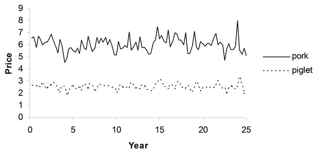
Figure 3. Price dynamics for  and
and 
 .
.
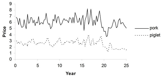
Figure 4. Price dynamics for  and
and 
 .
.
such as a certain transmission of price fluctuations of the final product. In a real options environment this uncertainty may cause investment reluctance on the different steps of the production chain. This paper analyses whether stronger vertical integration along the production chain reduces investment reluctance. For this purpose an agent-based competitive model of production chains was developed in which firms use optimal investment strategies identified by genetic algorithms. Two production systems were compared: As an example of a perfectly integrated system, it was considered that every firm can invest in closed systems in which the intermediate productand the final product are produced in equal amounts. In an alternative production system, firms can either invest in the intermediate product or the final product. The intermediate product is traded on a spot market.
Our simulations showed that the spot market solution and the closed system lead to practically the same production dynamics. The only precondition is that for the spot market system, producers of the intermediate product and producers of the final product have a good guess of the investment strategies and production capacities of other producers. This general finding is independent of different depreciation rates of the production steps, though the price dynamics for the intermediate product is strongly affected by the relation of depreciation rates on the different levels of the chain.
At first glance, our results may be intuitively surprising, but this is in accordance with several other surprising insights provided by the real options theory, for example, that myopic investors who ignore the impacts of competition behave efficiently ([5]) or that real options theory does not justify price stabilization policies ([27]).
5. Acknowledgements
The authors gratefully acknowledge financial support from the German Research Foundation (DFG) through research unit 986 “Structural Change in Agriculture” (SiAg).
REFERENCES
- C. Henry, “Investment Decisions under Uncertainty: The ‘Irreversibility Effect’,” The American Economic Review, Vol. 64, No. 6, 1974, pp. 1006-1012.
- B. S. Bernanke, “Irreversibility, Uncertainty, and Cyclical Investment,” Quarterly Journal of Economics, Vol. 98, No. 1, 1983, pp. 85-106. doi:10.2307/1885568
- R. McDonald and D. Siegel, “The Value of Waiting to Invest,” Quarterly Journal of Economics, Vol. 101, No. 4, 1986, pp. 707-727. doi:10.2307/1884175
- R. S. Pindyck, “Irreversibility, Uncertainty, and Investment,” Journal of Economic Literature, Vol. 29, No. 3, pp. 110-1148.
- J. V. Leahy, “Investment in Competitive Equilibrium: The Optimality of Myopic Behavior,” Quarterly Journal of Economics, Vol. 108, No. 4, 1993, pp. 1105-1133. doi:10.2307/2118461
- S. R. Grenadier, “The Strategic Exercise of Options: Development Cascades and Overbuilding in Real Estate Markets,” The Journal of Finance, Vol. 51, No. 5, 1996, pp. 1653-1679. doi:10.1111/j.1540-6261.1996.tb05221.x
- S. R. Grenadier, “Option Exercise Games: An Application to the Equilibrium Investment Strategies of Firms,” The Review of Financial Studies, Vol. 15, No. 3, 2002, pp. 691-721. doi:10.1093/rfs/15.3.691
- R. Novy-Marx, “An Equilibrium Model of Investment under Uncertainty,” The Review of Financial Studies, Vol. 20, No. 5, 2007, pp. 1461-1502. doi:10.1093/revfin/hhm013
- K. S. Pietola and H. H. Wang, “The Value of Price and Quantity Fixing Contracts,” European Review of Agricultural Economic, Vol. 27, No. 4, 2000, pp. 431-447. doi:10.1093/erae/27.4.431
- J. Arifovic, “Genetic Algorithm Learning in the Cobweb Model,” Journal of Economic Dynamics and Control, Vol. 18, 1994, pp. 3-28. doi:10.1016/0165-1889(94)90067-1
- J. H. Feil, O. Musshoff and A. Balmann, “Policy Impact Analysis in Competitive Agricultural Markets: A Real Options Approach,” European Review of Agricultural Economics, 2013. doi:10.1093/erae/jbs033
- N. J. Vriend, “An Illustration of the Essential Difference between Individual and Social Learning, and Its Consequences for Computational Analyses,” Journal of Economic Dynamics and Control, Vol. 24, No. 1, 2000, pp. 1-19. doi:10.1016/S0165-1889(98)00068-2
- A. Balmann and O. Musshoff, “Real Options and Competition: The Impact of Depreciation and Reinvestment,” Paper Presented at EAAE Congress, 28-31 August 2002, Zaragoza.
- S. Russel and P. Norvig, “Artificial Intelligence: A Modern Approach,” Prentice-Hall, Upper Saddle River, 1995.
- J. H. Holland, “Adaptation in Natural and Artificial Systems,” The University of Michigan Press, Ann Arbor, 1975.
- D. E. Goldberg, “Genetic Algorithms in Search, Optimization, and Machine Learning,” Addison-Wesley, Reading, 1989.
- S. Forrest, “Genetic Algorithms: Principles of Natural Selection Applied to Computation,” Science, Vol. 261, No. 5123, 1993, pp. 872-878. doi:10.1126/science.8346439
- M. Mitchell, “An Introduction to Genetic Algorithms,” MIT-Press, Cambridge, 1996.
- J. Arifovic, “The Behavior of the Exchange Rate in the Genetic Algorithm and Experimental Economies,” Journal of Political Economy, Vol. 104, No. 3, 1996, pp. 510- 541. doi:10.1086/262032
- R. Axelrod, “The Complexity of Cooperation. AgentBased Models of Competition and Collaboration,” Princeton University Press, Princeton, 1997.
- H. Dawid, “Adaptive Learning by Genetic Algorithms: Analytical Results and Applications to Economic Models,” Lecture Notes in Economics and Mathematical Systems, No. 441, Springer, Berlin, 1996.
- H. Dawid and M. Kopel, “The Appropriate Design of a Genetic Algorithm in Economic Applications Exemplified by a Model of the Cobweb Type,” Journal of Evolutionary Economics, Vol. 8, No. 3, 1998, pp. 297-315. doi:10.1007/s001910050066
- “Production costs and margins of pig fattening farms, 2008 Report,” European Commission, Directorate-General for Agriculture and Rural Development, Microeconomic Analysis of EU Agricultural Holdings, 2009.
- “2009 Pig Cost of Production in Selected Countries,” Agriculture and Horticulture Development Board, 2010.
- M. Odening, O. Musshoff, N. Hirschauer and A. Balmann, “Investment under Uncertainty—Does Competition Matter?” Journal of Dynamics and Control, Vol. 31, No. 3, 2007, pp. 994-1014. doi:10.1016/j.jedc.2006.03.005
- J. L. Lusk, T. L. Marsh, T. C. Schroeder and J. A. Fox, “Wholesale Demand for USDA Quality Graded Boxed Beef and Effects of Seasonality,” Journal of Agricultural and Resource Economics, Vol. 26, No 1, 2001, pp. 91- 106.
- A. Dixit and R. S. Pindyck, “Investment under Uncertainty,” Princeton University Press, Princeton, 1994.
Appendix
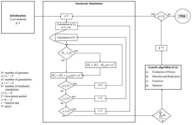
Figure A1. Flow diagram of the agent-based simulation approach.
NOTES
1Note that  is zero if there is no investor in period t.
2This formation of expectations is a slight deviation of the rational expectations assumption. Alternatively, it can be assumed that intermediate producers are perfectly aware of the investment strategies of final producers, and vice versa. This would lead to identical prices of the final product as in the perfectly integrated system and thus to identical investment triggers. The introduction of adaptive expectations can therefore be understood as some boundedly rational behaviour.
3The figures are within the same range as those reported by [23,24].
4If we would consider that piglet and pork producers would be perfectly aware of the investment behaviour of each side, identical trigger prices for closed systems and market interaction would be achieved.
5E.g., [26] obtained an elasticity of demand for pork of −0.47.