Open Journal of Safety Science and Technology
Vol.2 No.2(2012), Article ID:20268,6 pages DOI:10.4236/ojsst.2012.22006
Modelling of Fatigue-Type Seismic Damage for Nuclear Power Plants
Nuclear Power Plant Paks Ltd., Paks, Hungary
Email: katonat@npp.hu
Received February 25, 2012; revised March 24, 2012; accepted April 2, 2012
Keywords: Seismic Fragility; Cumulative Absolute Velocity; Fatigue
ABSTRACT
Assessment of seismic safety of the nuclear power plants requires knowledge of plant fragilities. In the paper, preliminary analysis is made on use of the cumulative absolute velocity in modelling of fatigue-type seismic damage. The dependence of the cumulative absolute velocity on the strong motion parameters is analysed. It is demonstrated that the cumulative absolute velocity is an appropriate damage indicator for fatigue failure mode. Failure criteria are defined in terms of cumulative absolute velocity using various fatigue failure theories.
1. Introduction
One of the most complex cases for assessing the nuclear power plant safety is the evaluation of the response of the plant to earthquakes and the risk related with this. It has to be demonstrated, whether the reactor can be shut down, cooled-down, the residual heat can be removed from the core, and the radioactive releases can be limited below the acceptable level. Well-defined set of plant systems and structures and components (SSCs) are required to be functional during and after the earthquake for ensuring these basic safety functions.
For the design base earthquake, the basic safety functions have to be ensured in deterministic sense, via adequate design supported by the proper definition of the parameters of the safe shutdown earthquake.
For quantification of safety, the annual core damage frequency with respect to earthquakes is calculated by probability safety analysis (PSA) using well-established procedures, see [1,2]. Event trees are constructed to simulate the plant system response. Fault trees are needed for the development of the probability of failure of particular components taking into account all failure modes. The hazard is expressed by the probability distribution for the peak ground acceleration (PGA). The fragility is defined as the conditional probability of damage as a function of PGA.
According to the results of the seismic probabilistic safety assessment of plenty of nuclear power plants, the earthquakes can be the dominating contributors to the core damage probability. These results indicate the vulnearbility of the plants against earthquakes. On the other hand, experiences show that plants survive much larger earthquakes than those considered in the design base, as it was the case of Kashiwazaki-Kariwa NPP, where the safety classified structures, systems and components survived the Niigata-Chuetsu-Oki earthquake in 2007 without damage and loss of function [3]. In spite of the nuclear catastrophe of the Fukushima Daiichi plant caused by the tsunami after Great Tohoku earthquake 11th of March 2011, the behaviour of thirteen nuclear units in the impacted area demonstrated high earthquake resistance.
With respect to the seismic safety of the operating plants the practical questions to be answered are:
• Whether the operation can be continued safely after a relative small earthquake. This is the issue of the Kashiwazaki-Kariwa plant which was shutdown for long-term after the earthquake in 2007.
• In case of large earthquake, the damaged condition of the plant has to be assessed for the emergency management reasons. This is the case of the Fukushima plants.
Experience shows that the design basis capacity expressed in terms of PGA does not provide direct information on the occurrence of a failure of a SSC in case of a particular earthquake.
A study performed by EPRI regarding failure indicators demonstrated that the cumulative absolute velocity (CAV) could be better correlated to damage rather than the PGA [4]. The EPRI study validates the lower bound of standardized CAV for damage of non-engineered structures.
Based on the EPRIS study, the U.S. NRC Regulatory Guide 1.166 defines the criteria for exceedance of operational base earthquake level. Recently, a coordinated research programme of the International Atomic Energy Agency is addressing the selection/development of appropriate damage indicators for nuclear power plants.
In [5] considerations were given on the possibility for derivation of conditional probability of failure for cumulative absolute velocity instead of peak ground acceleration. A physical interpretation of the cumulative absolute velocity and its dependence on strong motion parameters and load characteristics relevant for damage indication are discussed in [6]. It is also shown in [6], why the cumulative absolute velocity is an appropriate damage indicator especially for the fatigue-type damage.
In this paper, the cumulative absolute velocity—which is some kind of measure of the energy of the ground motion obtained from the free-field record—is expressed as a function of basic characteristics of the ground motion, i.e. strong motion duration and power spectra. The CAV will be linked to the stress or strain amplitudes and cycles affecting the component and causing fatigue type damage. With respect to the earthquake damage, different types of fatigue mechanisms can be considered, e.g. the fatigue racheting, low-cycle fatigue. Relation between cumulative absolute velocity of failure and failure criteria of various failure theories, e.g. fatigue failure condition the Bendat narrow-band theory and Dirlik formulation of the random amplitude fatigue failure, and the crack-growth condition has been established in the paper.
2. The CAV as Fragility Parameter
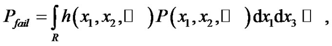
The probability of damage/failure, Pfail depends on a load vector  rather than on a single parameter:
 (1)
(1)
where  represents the hazard, i.e. it is the probability density function of applied loads and
  denotes the conditional distribution function of failure.
This approach might seem theoretically precise, however definition of the dependence of fragility on the components of the load vector requires enormous effort. The characterization hazard should also correspond to the description of fragility.
As it is shown in [4], it seems to be interesting to establish a method for fragility modelling based on use of CAV as a nonnegative single load parameter x ≥ 0. CAV is calculated as simple integral over the time history of absolute value of acceleration component:
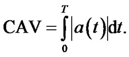 (2)
(2)
The standardized CAV is calculated applying a noisefilter for the amplitudes less than ±0.025 g [5].
For the sake of simplicity of writing, CAV will be denoted below simple by x. Equation (1) can be rewritten as follows:
 (3)
(3)
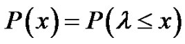
Assuming that, if a failure occurs for a value of CAV equal to x, then it is occurs for all values larger than x. In this case the conditional probability distribution function P(x) coincides with the cumulative probability distribution function of the failure load parameter λ, i.e. of the smallest value of the load parameter that the structure is unable to withstand [4],
 (4)
(4)
From the equation above, the average value of the failure load parameter can be calculated. The average CAV-value of failure:
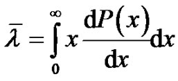 (5)
(5)
With other words, for the effective use of CAV in fragility analysis, the value λ has to be evaluated from the empirical data (damages of earthquakes, fragility tests) for all type of SSCs and failure modes.
3. The Physical Meaning of the CAV
As it has been shown in [4], the value of CAV is varying within a wide range depending on several parameters of the ground motion: PGA, duration, T, and frequency content of the random motion. However, these dependences, except for the dependence on T, are not obvious and not explicit. It is reasonable to define the dependence of the CAV on the strong motion parameters.
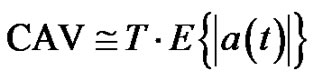
The absolute value of the acceleration (or the component of the acceleration)  is an integrable function and its mean value on T is equal to
 . Thus, the mean value theorem for the integral can be applied for the Equation (2) as follows:
 (6)
(6)
Thus, the CAV can be considered as product of two random variables, the duration of strong motion T and the mean of absolute value of ground acceleration time history. Generally, the variables T and  might not be independent.
The strong motion acceleration time history can be written in form: a(t)=I(t)x(t), where I(t) is a windowfunction on [0, T] interval, i.e., I(t) º 0 if t = 0 and t = T and outside of interval and I(t) > 0 within the interval. It is assumed that x(t) is a stationary normal random process. However, the a(t) is a non-stationary normal process. For the sake of simplicity let’s assume that a(t) is a stationary normal random process with zero mean and probability density function fa(a) and autocorrelation function R(t). In this case, the random process z(t) = |a(t)| has the density function, fz(z) = 2fa(z)·U(z), and its mean value is as follows [7]:
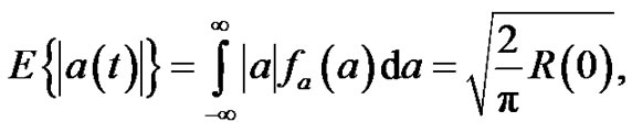 (7)
(7)
where R(0) is the autocorrelation function of a(t) at t = 0. The R(0) can be rewritten as follows:
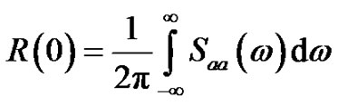 (8)
(8)
where Saa(ω) is the power spectral density (PSD) function of a(t).
The power spectral density function Saa(ω) of the earthquake ground motion acceleration is showing bandlimited or even narrow-band character. Since we intend to explain the qualitative features of the CAV we may assume that a(t) is an ideal band-limited process with power spectral density (PSD):
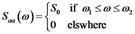 (9)
(9)
This assumption is based on NUREG-0800, where the one-sided PSD of the horizontal ground motion acceleration time history is linked to the Regulatory Guide 1.60 standard response spectrum.
Assuming that the excitation energy is concentrated within a narrow frequency range, the R(0) can be written as follows:
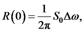 (10)
(10)
where  is the bandwidth. The Equation (6) we can rewrite as follows:
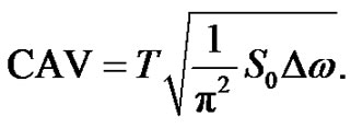 (11)
(11)
Introducing the median frequency ωc:
 (12)
(12)
and the number of load cycles, N
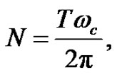 (13)
(13)
the CAV can also be expressed as follows:
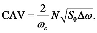 (14)
(14)
If the a(t) is band-limited we can represent it with sum of sine functions:
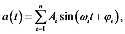 (15)
(15)
and the energy of a(t) should be distributed as follows:
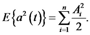 (16)
(16)
For the amplitudes Ai in dw intervals at ωi the following equation is valid:
 (17)
(17)
For the sake of simplicity the excitation can be represented by a single sine with median frequency ωc and , thus for the CAV the following simple equation can be obtained:
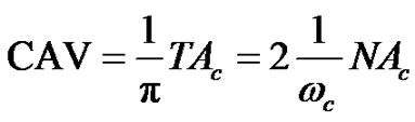 . (18)
The following conclusion can be drawn:
• The CAV is proportional to the product of strong motion duration and average energy (RMS) of the strong motion acceleration a(t), as it shown by Equation (6). This result is rather trivial.
• The CAV should be an adequate damage indicator since it is correlated to the main parameters of damage phenomena, i.e. to the number of load cycles, N, and median frequency, wc and amplitude of the alternating load, which is proportional to the ground motion acceleration amplitude, i.e. Ac.
• The higher the mean frequency of the excitation is, the less will be the possibility of a damage at fixed value of N, which corresponds to the observations for large class of structures with low frequencies.
4. CAV as Fatigue Failure Indicator
Several damage mechanisms might be in place due to cyclic earthquake loads, e.g. fatigue racheting, low-cycle fatigue.
A straightforward calculation of the fatigue damage to a structure consists of three basic steps:
1) Calculate the (nonlinear) time-history response of the structure to an earthquake loading.
2) Convert the time history response to an equivalent series of loading cycles.
3) Calculate the fatigue damage of the equivalent cyclic responses.
Fatigue damage estimation involves the cycle counting of equivalent stress ranges and accumulation of fatigue damage from each cycle. The seismic loads are not made up of complete, consistent cycles. Typical seismic response time histories exhibit varying amplitudes, mostly partial cycles, and no complete symmetric cycles. In this case, after estimating an equivalent stress range distribution either in the time domain or in the frequency domain, the linear Palmgren-Miner rule is used to predict the damage per cycle as
 (19)
(19)
where Di is the damage for cycles of magnitude i, and Nfi is the number of cycles to failure at level i. The total damage over the complete cycling history is then estimated as
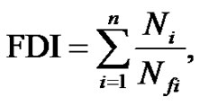 (20)
(20)
where FDI is the fatigue damage index, or total damage to the element due to the cyclic load, n is the number of different cycle amplitudes in the loading history, and Ni is the number of cycles at amplitude i. Values of FDI greater than or equal to 1.0 indicate a low-cycle fatigue fracture of the structure.
In order to use the measured seismic response to calculate fatigue damage, it is necessary to convert the load time history to a series of varying amplitude cycles. The rain-flow method is most commonly used for converting random stressors to cycles.
Let’s consider a free-field mounted one-degree-offreedom (ODF) structure, with m, mass, k, stiffness, c, damping, ω0, resonance frequency,  , and transfer function
  . Assuming linear stress strain relationship, the stress level s(t) is directly proportional to the relative displacement level z(t), i.e. s(t) = k·z(t), where k is a constant. Calculating the relative displacement response of the ODF system to the sinusoidal excitation with
 , the stress level can be defined. Standard fatigue model might be applied for the definition of the number of cycles to failure for the calculated stress amplitude. For the ODF system, the CAV to fail can be calculated using Equation (18).
In the case of generic base acceleration excitation a(t), the response of the ODF in terms of stress level will be
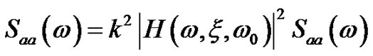 (21)
(21)
Equation (21) can be generalised introducing the transfer function  between ground motion acceleration a(t) and any response quantity of interest, y (e.g. stress, strain, displacement):
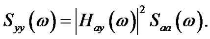 (22)
(22)
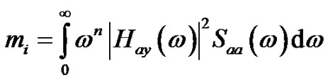
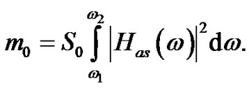
For the definition of the fatigue failure, the moments mi of the power spectral density of the stress history Sss(ω) have to be calculated:
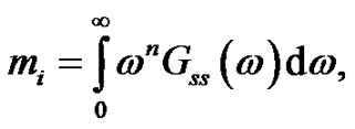 (23)
(23)
where Gss(ω) is the one-sided PSD corresponding to Sss(ω). Thus, the following equations can be written:
for the root-mean-square value  for the zero-crossing, E[0]:
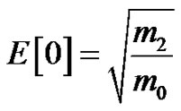 (24)
(24)
for the peak-rate, E[P]:
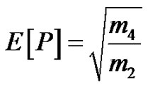 (25)
(25)
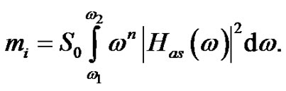
Utilising Equation (22) and assuming narrow-band feature for ground motion acceleration, as it is expressed by the Equation (9), Equation (23) can be rewritten as follows:
 (26)
(26)
 (27)
(27)
For the RMS the following Equation can be derived:
 (28)
(28)
It means that except for the RMS all interested values, i.e. the E[0] and E[P] are independent from the excitation, S0.
For the calculation of fatigue failure condition, the Bendat narrow-band theory can be used [8]. It is assumed, that the probability density function of the peaks for the narrow band signal can be approximated by Rayleigh distribution. Thus, the FDI can be calculated as follows:
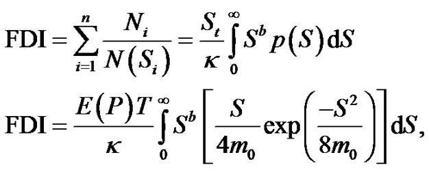 (29)
(29)
where N(Si) is the number of cycles of stress range S occurring in T seconds, Ni is the actual counted number of cycle, St = N, the total number of cycles equals to  , E[P] is the number of peaks per second. Parameters κ and b are the materials constant defining the fatigue curve. In the Equation (29), the m0 is depending on the input excitation power spectral density function, which is assumed to be equal to S0.
In the Equation (29), the m0 can be expressed using Equation (11). Thus, the relation between CAV and fatigue failure condition is established.
Similarly, the Dirlik solution [9] for the p(S) probability density function can be linked to the CAV of ground motion exciting the structure. The number of stress cycles of range N(S) can be calculated via:
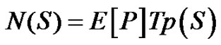 (30)
(30)
Dirlik solution for the probability density function is as follows:
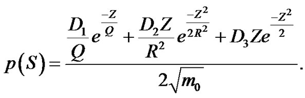 (31)
(31)
where D1, D2, D3, R are parameters depending on m0, m1, m2 and m4, but not depending on the input excitation power spectral density, if the excitation is narrow-band.
The Z is depending on the RMS of the input excitation only, which can be expressed by CAV via Equation (11). Thus, the final results of the calculation of the fatigue failure can be correlated to the cumulative absolute velocity of the ground motion excitation.
There are other fatigue failure theories, which can be correlated to the ground motion excitation via CAV. Assuming that the failure mode is the low-cycle fatigue, the well-known Coffin-Manson relation for low-cycle fatigue can be written
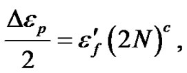 (32)
(32)
where  is the plastic strain amplitude,
  is the fatigue ductility coefficient, 2N is the number of reversals, or simple the N cycles, and c is an empirical constant ranging from –0.5 to –0.7.
For the sake of simplicity the excitation can be written as a single sine with median frequency ωc, and 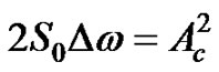 . The stress amplitude will be as follows:
 (33)
(33)
where  is the absolute value of the accelerationstress transfer function.
The CAV to fail can be written using Equation (18) as follows:
 (34)
(34)
Thus, the CAV to fail is connected to the failure criteria due to the low-cycle fatigue.
Failure of a material due to fatigue may be viewed on a microscopic level. The first phase is the crack initiation. The second phase is the crack propagation. The final phase is the failure. For example, the Newman’s stress intensity solution can be used to calculate the RMS stress intensity factor range ΔKRMS
 (35)
(35)
where b is the crack depth and Q is the elastic shape factor for an elliptical crack, and Me is the elastic magnification factor (see e.g. [10]). The maximum and minimum stress RMS values can be calculated utilising the moments of the power spectral density function of the stress response, see Equation (23). The latter can be linked to the power spectral density of the excitation via Equation (22).
There are several important aspects and theories of the fatigue not considered in the paper. Development of a failure mechanism is time dependent. Consequently, the description of deterioration should also be time-dependent. The process of progressing damage can be modelled as first-passage problem, i.e. failure occurs when the margin to the limit state, which is also time dependent, will be first time zero (see e.g. [11,12]).
Obviously, a comprehensive analysis of the use of CAV and establishing the exact relationship between CAV and typical fatigue mechanisms and corresponding theories need further research effort.
5. Conclusions
Reliable methods for justification of the safety are needed for the cases, when earthquake hits the plants. Development of the fragility of SSCs for different failure modes is one of the basic issues of the evaluation of the seismic safety of nuclear power plants. Sparse statistical information exists on behaviour of complex structures/machines under earthquake loads. Fragility test of components might be very expensive. Epistemic uncertainty in the failure modelling might be substantial.
In the seismic PSA practice, the component fragility development is based on the design information anchored into PGA. Use of the cumulative absolute velocity as load parameter may improve the calculation of probability failure.
It is also shown in the paper, that the CAV is reflecting both the main parameters of the fatigue process and characteristics of the earthquake excitation. The CAV can be correlated to the failure criteria defined via different methodologies for random amplitude, frequencydomain fatigue analysis, as well as to the low-cycle fatigue failure criteria. It is shown, that a correlation between CAV and stress intensity factor range can also been established.
Having these correlations established in advance, the condition of the equipment can be assessed if an earthquake happen, which may contribute to the quick assessment of the plant safety after an earthquake.
Obvious advantage of the use of the CAV for damage indicator is that it can be calculated nearly real-time from the easy to measure free-field acceleration signal.
At the present stage of the research, the paper demonstrates more an attempt for improving the seismic safety assessment of nuclear power plants rather than a comprehensive study. Considering the importance of the seismic safety of the nuclear power plants, it is believed that the problem addressed in this paper is highly challenging and the issues presented are worth for more research work in the future.
REFERENCES
- R. P. Kennedy and M. K. Ravindra, “Seismic Fragilities for Nuclear Power Plant Risk Studies,” Nuclear Engineering and Design, Vol. 79, No. 1, 1984, pp. 47-68. doi:10.1016/0029-5493(84)90188-2
- ANSI/ANS-58.21-2003: External Events PRA Methodology, 2003.
- IAEA, “Preliminary Findings and Lessons Learned from the 16 July 2007 earthquake at Kashiwazaki-Kariwa NPP,” Mission Report, 2007.
- Electrical Power Research Institute, “A Criterion for determining Exceedance of the Operating Basis Earthquake,” EPRI Report NP-5930, 1988.
- T. Katona, “Options for the Treatment of Uncertainty in Seismic Probabilistic Safety Assessment of Nuclear Power Plants,” Pollack Periodica, Vol. 5, No. 1, 2010, pp. 121- 136. doi:10.1556/Pollack.5.2010.1.9
- T. J. Katona, “Interpretation of the Physical Meaning of the Cumulative Absolute Velocity,” Pollack Periodica, Vol. 6, No. 1, 2011, pp. 99-106.
- A. Papoulis, “Probability, Random Variables, and Stochastic Processes,” McGraw-Hill, New York, 1965.
- J. S. Bendat, “Probability Functions for Random Responses,” NASA report on Contract NAS-5-4590, 1964.
- T. Dirlik, “Application of computers in Fatigue Analysis,” Ph.D. Thesis, University of Warwick, Coventry, 1985.
- S. T. Kim, D. Tadjiev and H. T. Yang, “Fatigue Life Prediction under Random Loading Conditions in 7475T7351 Aluminum Alloy using the RMS Model,” International Journal of Damage Mechanics, Vol. 15, No. 1, 2006, pp. 89-102.
- O. Ditlevsen, “Random Fatigue Crack Growth—A FirstPassage Problem,” Engineering Fracture Mechanics, 1986, Vol. 23, No. 2, pp. 467-477. doi:10.1016/0013-7944(86)90088-3
- P. H. Wirsching, H. P. Nguyen and K.-T. Ma, “Fatigue Reliability as a First Passage Problem,” 8th ASCE Specialty Conference on Probabilistic Mechanics and Structural Reliability, Notre Dame, 24-26 July 2000.