Open Journal of Ecology
Vol. 3 No. 2 (2013) , Article ID: 30962 , 11 pages DOI:10.4236/oje.2013.32010
A study of using grey system theory and artificial neural network on the climbing ability of Buergeria robusta frog
![]()
1Department of Landscape and Architecture, Mingdao University, Chanhua, Chinese taipei
2Department of Design for Sustainable Environment, Mingdao University, Chanhua, Chinese taipei; *Corresponding Author: tfchuang@mdu.edu.tw
Copyright © 2013 Yuan-Hsiou Chang, Tsai-Fu Chuang. This is an open access article distributed under the Creative Commons Attribution License, which permits unrestricted use, distribution, and reproduction in any medium, provided the original work is properly cited.
Received 25 February 2013; revised 3 April 2013; accepted 23 April 2013
Keywords: Ecological Engineering; Artificial Neural Network; Grey System Theory; Buergeria robusta
ABSTRACT
Ecological engineering is an emerging study of integrating both ecology and engineering, concerned with the design, monitoring, and construction of ecosystems. In recent years, the threat to amphibian animals is becoming more and more serious. In particular, the loss of habitats caused by changes to the way land is used by human beings has hit amphibians particularly hard. Amphibians are known to be particularly vulnerable to human activities because they rely on both terrestrial and aquatic habitats for survival. With the increasing development of many areas in recent years, concrete structures are often installed along water bodies in order to increase the safety of local residents. The construction of concrete banks along rivers associated with human development has become a serious problem in Taiwan. Most ecosystems used by amphibians are lakes and stream banks, yet no related design solutions to accommodate the needs of amphibians. The need to develop the relevant design specification considering protecting the amphibian is imperative. Buergeria robusta, an endemic species in Taiwan, is tree frog widely distributed in lowland montane regions. Their breeding season is from April to September. They like to rest on trees or hide at caves during the daytime and move to the stream nearby in dusk for breeding. Males usually emit weak mating call while standing on stones. Sticky eggs are attached to undersides of rocks and stones. Tadpoles are found in slow flowing water of streams [1]. The goal of this study is to improve the understanding of the relationship between the climbing ability and the physical characteristics of amphibians. In this study, we use Artificial Neural Network to simulate the climbing ability of Buergeria robusta. Besides, Grey System Theory is also adopted to improve the performance of Artificial Neural Network. Artificial Neural Network (ANN) is a computing system that uses a large number of artificial neurons imitating natural neural ability to deal with an information network by computing system. The numerical results have show good agreement with the experimental results. The results can serve as a reference for technicians involved in future ecological engineering designs of banks throughout the world.
1. INTRODUCTION
Taiwan is a continental island, located between the southeastern coastline of mainland China and Japan's Ryukyu Islands. With diverse terrain and wide range of vertical elevations, Taiwan has tropical, subtropical, temperate, and frigid climate zones. These unique geographical conditions, coupled with the effect of habitat isolation, gave Taiwan its high biodiversity [2].
The emerging discipline of ecological engineering is a response to the growing need for engineering practices to provide for human welfare while at the same time protecting the natural environment from which goods and services are drawn [3]. According to Mitsch [4], the meaning of Ecological engineering is “the design of sustainable ecosystems intends to integrate human society with its natural environment for the benefit of both.”
The increase of human population is transforming many native environments into human-dominated landscapes. Environmental impacts of human activities are readily apparent, causing dramatic changes in patterns of species composition, abundance, and diversity in various ecosystems [5-9].
In recent years, the major concern has been focused on the global decline of many amphibian populations [10-17]. It is well known that habitat destruction is the major cause of amphibian extirpations, and many amphibian species are currently under-going population declines, range reductions, and even extinction [18] Declines in amphibians could have a critical impact on other organisms due to their contribution to trophic dynamics in both terrestrial and aquatic communities. Researchers in many countries have attempted to investigate the reasons of decreasing amphibian populations, and seek possible solutions to manage and restore their habitats [19-22].
Amphibians have long played important roles in Taiwanese ecosystems [23-26]. Because amphibians live both in water and on land, the quality of bank between these two areas is crucial to their survival. In recent years, threats to amphibian habitat, such as concrete being applied as a construction material on lakeshores, have become increasingly serious. These threats have resulted in alterations of the habitats on which amphibians rely. However, very little research considering the effect of these structures on the decline of amphibian populations in Taiwan has been performed.
Hou et al. [25] used endemic species, Chirixalus idiootocus, as an indicator to understand the relationship between amphibian behavioral capacity and environment factors. They found that substrates and weather conditions are important factors in the activity of C. idiootocus, and indicated that more comprehensive studies and experiments involving different species should be performed to further examine how local climate and lakeshore and stream bank conditions affect activities of amphibians. This will lead to better management of river banks, especially when considering the degree to which many urban rivers are modified.
Chang et al. [27] selected eight species of amphibians and investigated their climbing abilities in an effort to improve lake and river bank designs. They evaluated their climbing abilities on five angles of bank slopes, identified relationships between an amphibian’s climbing ability and different surface substrates of banks, i.e. Japanese silvergrass (Miscanthus floridulus) mixed with moss, cobblestone, wood (Philippine mahogany), clay, and concrete, under high humidity and different temperatures to simulate changes across the four seasons.
The major objective of this study is to improve the understanding of the climbing abilities of amphibians. An endemic species, Buergeria robusta, was chosen to investigate whether the climbing abilities can be estimated by using the physical characteristics of amphibians. In this paper, we used Artificial Neural Network to simulate the climbing ability of Buergeria robusta. Besides, Grey System Theory [28] is also adopted to improve the performance of Artificial Neural Network. The results could provide a useful material for engineers involved in future engineering of aquatic banks, and to suggest substrates and inclines that will promote amphibian conservation and habitat management.
2. MATERIALS AND METHODS
2.1. Sampling and Grouping
In this study, a Taiwan endemic species, Buergeria robusta, was chosen for investigation. In particular, this frog was a protected species in Taiwan before 2008 mainly due to the habitat loss. Although the amount of this amphibian has increased these years, it is still necessary to collect sufficient materials in order to protect their habitat. Sample numbers and measurement periods were determined based on patch and on-site sampling methods proposed by Lue [23]. Using the Amphibians Resource Survey Handbook [23], the quantitative requirements of biological sampling were adopted for field tests [29].
30 male and 10 female frogs were gathered in Wulai Distribution (located at north of Taiwan). The 40 collected creatures were numbered and kept in aquariums. Since the creatures’ behavioral capacity may be affected by long-term laboratory observations [23,29], the subsequent laboratory experiments were performed within 14 days after the capture of the creatures. All the creatures were then returned to the original site after the experiments were completed.
2.2. Experiment
The body height, weight, high jump and long-jump ability were measured and recorded (as shown in Table 1) before grouping. An electronic scale and a Vernier caliper were used to measure the samples’ body weights and straight body lengths, respectively. Jumping heights were measured using paper tubes of diameters ranging from 5 to 18 cm reeled from 1 mm thick cardboard, with heights ranging from 3 to 60 cm. The height difference between each paper tube was 2 cm. Using grass as a stimulus, five jumps were surveyed at 1 min intervals, and the average was calculated. Regarding the jumping length, the specimen was placed in a fixed position, on a 200 × 200 cm flat board, and then the mean distance of five long
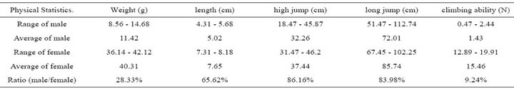
Table 1. Physical characteristics of frogs.
jumps was measured [26].
The climbing ability of the amphibians was tested using a simple apparatus [30] (Figure 1) and then divided by individual body weight (Table 1). The substrate is chosen to be Japanese silvergrass (Miscanthus floridulus) and the bank slope on amphibians’ climbing ability is chosen to be 15˚ in this pilot study [27]. Each organism was swathed in wet cloth and fastened to an electronic spring scale by a cotton string. The climbing ability was measured by pulling the scale gradually at 1 min intervals. The unit of measurement was N,and the mean value of five jumps were calculated. During all trials, the amphibian’s skin remained wet throughout the process.
The results (Table 1) showed that the physical characteristics and climbing ability between male and female frogs are quite different. For example, the average weight of the male frogs is 11.42 (g), while the value is 40.31 (g) for the female frogs. The ratio of average male weight to female weight is 28.33%. Besides, it can found that the jump ability and climbing ability performed by female frogs are better than male frogs. Due to the obvious differences between the male and female frogs, only the data of the male frogs have been chosen in the analysis of Artificial Neural Network.
2.3. Grey-Relational Analysis
The Grey theory established by Dr. Deng includes Grey relational analysis, Grey modeling, prediction and decision making of a system in which the model is unsure or the information is incomplete [29]. It provides an efficient solution to the uncertainty, multi-input and discrete data problem. The relation between machining parameters and machining performance can be found out using the grey-relational analysis. And this kind of interaction is mainly through the connection among parameters and some conditions that are already known. Also, it will indicate the relational degree between two sequences with the help of grey-relational analysis.
Grey-relational analysis [28] is mainly used to conduct a relational analysis of the uncertainty of a system model and the incompleteness of information. It can generate discrete sequences for the correlation analysis of such sequences with processing uncertainty, multi-variable
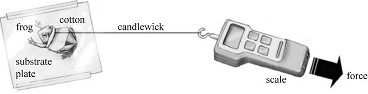
Figure 1. Apparatus for measuring climbing ability of a frog [26].
input and discrete data [31]. Consequently, grey-relational analysis is a measurement method to discuss the consistency of an uncertain discrete sequence and its target. In a given group for Grey relational analysis, all the sequences should comply with the comparability conditions of non-dimensional, scaling and polarization [28].
2.4. The Comparison of Sequence
Assure a sequence meets the following three conditions; this sequence is regarded to be comparable.
Non-dimensional: Factors must be processed to become non-dimensional.
Scaling: The values of each sequence belongs to the same order (order difference cannot be greater than 2)
Polarization: Factor description of sequence should be in the same direction.
2.5. Grey-Relational Generation
First, generate the measurement space factor from the original sequence factor in a process known as grey-relational generation [28]. This can be divided into three types: larger-the-better, smaller-the-better and nominalthe-better by characteristics.
Larger-the-better grey-relational generation: the maximum of the sequence factors is the ideal factor.
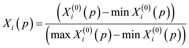 (1)
(1)
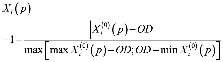
Smaller-the-better grey-relational generation: the minimum of the sequence factors is the ideal factor.
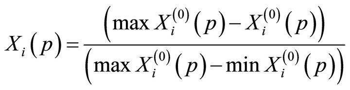 (2)
(2)
Nominal-the-better grey-relational generation: the one in line with the target value of the sequence factors is the ideal factor.
 (3)
(3)
where OD is the target value;  is the data after grey-relational generation;
  is the maximum value of the original sequence factor;
  is the minimum value of the original sequence.
2.6. Grey-Relational Degree
The grey-relational degree [28] is used to measure the correlation between the measurement space factor and reference sequence after a grey-relational generation of the discrete sequence. The grey-relational degree can be divided into two types of localized grey-relational degree and globalized grey-relational degree. This paper used the localized grey-relational degree in analysis.
Suppose that : the reference sequence,
  ;
; : the comparison sequences.
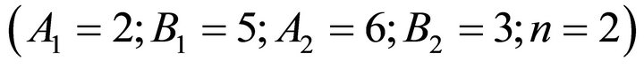
Assume each comparison sequence has m data and . Also assume there are n comparison sequences, where
 . The grey-relational coefficient is defined as
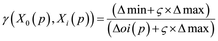 (4)
(4)
where : The absolute value of the minimum difference of the comparison sequence and the reference sequence;
 : The absolute value of the maximum difference of the comparison sequence and the reference sequence;
 : The absolute value of the difference of the comparison sequence and the reference sequence;
 : identification coefficient, [0; 1]: The main purpose of
  is to adjust the difference between
  and
and . Usually, this value is equal to 0.5.
Finally, the grey-relational grade is obtained by calculating the average value of the grey-relational coefficient for n comparison sequences is obtained as below:
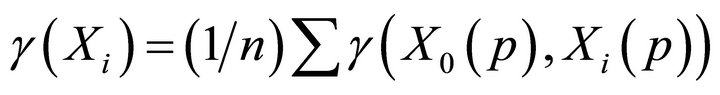 (5)
(5)
2.7. Grey-Relational Rank
After the grey-relational grade is calculated, we can rank the sequence based on the above values, and this procedure is called gray-relational rank [28]. If the two sequences are identically coincidence, then the value of grey relational grade is equal to 1. The grey relational grade also indicates the degree of influence that the comparability sequences could exert over the reference sequence. Therefore, if a particular comparability sequence is more important than the other comparability sequences to the reference sequence, then the grey relational grade for that comparability sequence will be higher than other grey relational grades. Grey analysis is actually a measurement of absolute value of data difference between sequences, and it could be used to measure approximation correlation between sequences.
2.8. Artificial Neural Network
Artificial Neural Network (ANN) [32] is a computing system that uses a large number of artificial neurons imitating natural neural ability to deal with an information network by computing system. It is composed of a large number of highly interconnected processing elements (neurones) working in unison to solve a specific problem. It is a technique that can analyze a large number of materials and build the relation between the input parameters and output terms [33], no matter whether the relationship is linear or non-linear. Therefore, it has wide application in many issues like optimization questions, distinguishing and classification, prediction models, and the approximate value of functions [34-36] indicated that the ANN method can model the nonlinear relationship between the input parameter and output terms.
The Back-propagation neural networks (BPNN), a branch of ANN, are neural networks capable of learning and recall. BPNN have been successfully applied in many areas, such as the analysis of biomechanics [37], analysis of computing muscular signals [38], and study of human gait patterns by adopting BPNN to distinguish leg length [39]. Wu et al. [40] suggested that the Back Propagation Neural Network (BPNN) is one of the most frequently utilized ANN methods for prediction because of its many advantages, including high learning accuracy, fast response, ease usability, and a capacity for dealing with complex and nonlinear data relationships. In general, the BPNN contains three parts, including one input layer, one or more hidden layers, and one output layer. The neurons in each layer are fully interconnected by connection strengths called weights which express the relative importance of each input to a processing element. The process of training a neural net-work involves adjusting weights to minimize the difference between the targets and the outputs. By repeating the learning process, the network learns the correct values of weights, finally obtaining the optimal outputs. The BPNN belongs to a multilayer feed-forward network, and its learning process usually adopted the steepest-descent method to amend weights and quickly minify errors to obtain the optimum function.
3. USING THE GRA TO IMPROVE THE BPNN
The procedure of using grey-relational analysis (GRA) to improve the accuracy of BPNN is shown below:
(1) Prepare the original data for grey-relational analysis
(2) Checking the comparability conditions needed for grey-relational analysis
(3) If the answer of item 2 is Yes, the original data can be used to proceed the grey-relational analysis.
(4) If the answer of item 2 is No, the data obtained from grey-relational generation can be used to proceed the grey-relational analysis.
(5) Calculate the grey-relational grade using Eq.5.
(6) Evaluate the grey-relational rank.
(7) Run BPNN and record the performance of network.
(8) Substitute the 5 neurons (4 neurons in the input layer and 1 neuron in the output layer) of Frog ID with the worse grey-relational rank for that with the better rank step by step, and run the BPNN again.
(9) Check whether the results of procedure (8) are better than those of procedure (7).
4. DESIGNING THE BPNN MODELS
4.1. Procedure of Designing BPNN Models
Designing BPNN models follows a number of procedures. Generally, there are four basics steps: 1) collecting data, 2) building the network, 3) train, and 4) test performance of model.
4.2. Building the Network
The network of this study was composed of three layers: input layer, hidden layer, and output layer (Figure 2). In this study, there were 4 neurons (Figure 3) in the input layer (height, weight, high jump and long-jump ability), and 1 neurons in the output layer (climbing ability per gram of body weight, 10−2 N/g). The number of neurons in that hidden layer is calculated in the following three ways: 1) the mean of the neurons in the input and output layers; 2) the sum of the neurons in the input and output layers; and 3) twice the sum of the neurons in the input and output layers. The MATLAB 7.0 software is used since it not only provides numerous ready-to-use algorithms for most methods of data analysis but also allows the existing routines to be modified and expanded.
4.3. Training the Network
During the training process, the weights are adjusted in order to make the actual outputs (predicated) close to the target (measured) outputs of the network. To prove that the BPNN had a good learning effect, the samples of
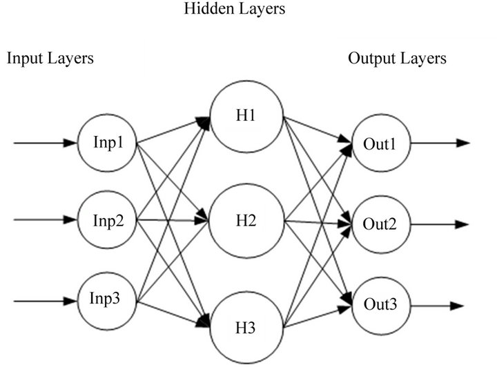
Figure 2. Back propagation neural networks.
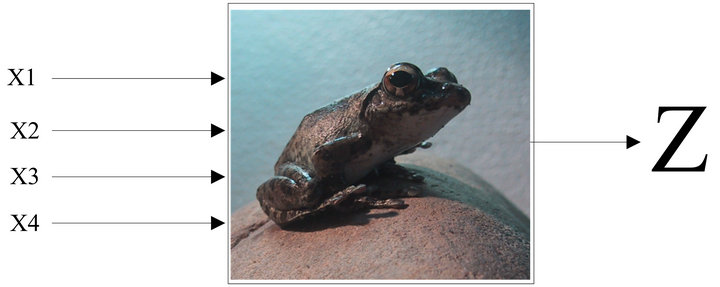
Figure 3. Network simulation of the frog’s behavior.
the subjects (frogs) were divided into two groups (training and testing samples) in ratios of 75:25. In the network, the training function available in Matlab 7.0 which adopted is the TRAINLM, adaption learning function is LEARNGDM, performance function is MSE, and the transfer function is TANSIG [41]. As can been seen in MATLAB User’s Guide that TRAINLM is a network training function that updates weight and bias values according to Levenberg-Marquardt optimization. LEARNGDM is gradient descent with momentum weight and bias learning function. MSE is a network performance function. It measures the network’s performance according to the mean of squared errors. TANSIG is hyperbolic tangent sigmoid transfer function [41].
4.4. Testing the Network
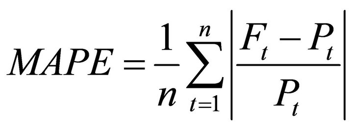
The next step is to test the performance of the developed model. At this stage unseen data are exposed to the model. In order to evaluate the performance of the developed BPNN models quantitatively and verify the accuracy in performance, the mean square error (MSE), the root mean square error (RMSE), the mean absolute error (MAE), and the mean absolute percentage error (MAPE) were adopted [42]. MSE provide information which is a measure of the variation of predicated values around the measured data. The lower the MSE, the more accurate is the estimation. MAE is a quantity used to measure how close forecasts or predictions are to the eventual outcomes. The lower the MAE, the more accurate is the estimation. The mean absolute percentage error (MAPE), also known as mean absolute percentage deviation (MAPD), is a measure of accuracy of a method which used the actual value as the denominator in the equation. This has made MAPE very easy to interpret and reflect the accuracy of the model.
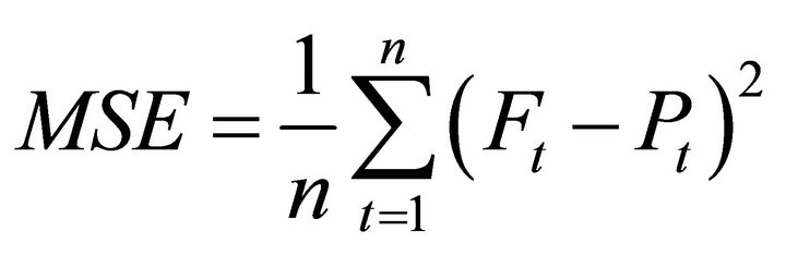 (6)
(6)
 (7)
(7)
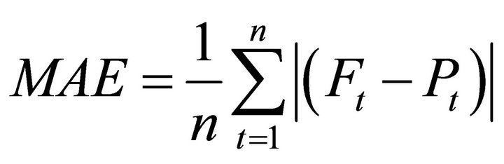 (8)
(8)
 (9)
(9)
where  is the forecast value and
  is the actual value.
5. NUMERICAL STUDY AND RESULTS
The weight, length, high jump, long jump and climbing ability of frogs obtained from experiment (Table 1) are chosen for grey-relational analysis and BPNN analysis. To satisfy the scaling of comparability condition, the original climbing ability is selected in the grey-relational analysis. It can be seen that the above original data has satisfied the comparability conditions (i.e. non-dimensional, scaling and polarization); therefore, the process of grey-relational generation is not necessary. In addition, as the localized grey-relational degree is adopted, the next step is to calculate reference sequence. In this study, the reference sequence was obtained using the average values of 30 male frogs (see Table 1). For example, the first value of reference sequence was 11.42 (see Table 2) which is the average weight of the 30 male frogs.
The results obtained by grey-relational analysis are shown in Tables 3-5. Table 3 shows the difference of the comparison sequence and the reference sequence. Table 4 shows the grey-relation grade calculated by using Eq.5. It can be seen that the minimum value of grey-relation grade is 0.7911 for frog No. 9 and the maximum value of grey-relation grade is 0.9468 for frog No. 28. Table 5 shows the grey-relational rank based on the above grey-relation grade. It can be seen that the Rank 1 is frog No. 28, Rank 2 is frog No. 13 and Rank 30 is frog No. 9.
As stated before, to prove that the BPNN had a good learning effect, the samples of the subjects (frogs) were divided into two groups (training and testing samples) in ratios of 75:25. As the total number of male frogs is 30, the number of frogs in the training and testing groups can be calculated to be 23 and 7, respectively. In order to understand whether the grey-relational analysis can im-
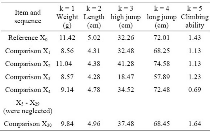
Table 2. Original data of grey-relational analysis.
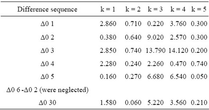
Table 3. The difference of the comparison sequence and the target sequence.
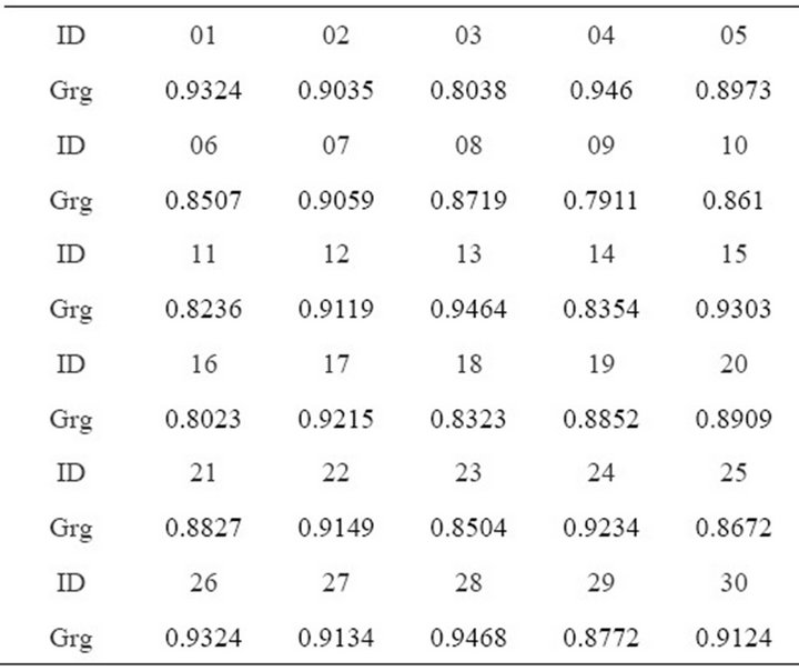
Table 4. Grey-relation grade of frog’s behavior.
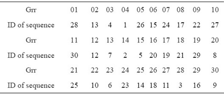
Table 5. Grey-relation rank (Grr) of frog’s behavior.
prove the accuracy of BPNN, the grey-relation ranks based on the total male frogs were re-ranked individually based on the training and testing groups.
Tables 6 and 7 show the new grey-relation ranks based on the training group (No. 1 - 23) and testing group (No. 24 - 30 frogs). Table 6 shows that Rank 1 is frog No. 13 (grey-relation grade is 0.9464), Rank 2 is frog No. 4 and Rank 23 is frog No. 9. Table 7 shows that Rank 1 is frog No. 28 (grey-relation grade is 0.9468), Rank 2 is frog No. 26 and Rank 7 is frog No. 25.
After the grey-relational analysis is completed, the next step is to investigate the performance of the developed BPNN models. Tables 8 and 9 showed the computed values of MSE, RMSE, MAE and MAPE for the developed BPNN models considering different network structures of samples. For the network structure identification used in the fourth column of Tables 8 and 9, the first number indicates number of neurons in the input layer, the last number represents neurons in the output layer, and the numbers in between represent neurons in the hidden layer.
During the training process, we noted that model 1 seems to be the best (see Table 8) among the three investigated BPNN models (model 1 - 3) as it yields the lowest values of MAPE (0.005341). Figure 4 gives further evidence that model 1 is the best among the three models.
During the testing process, again, we can see that model 1 (see Table 9 and Figure 5) is the best among the three models as it yields the lowest values of MSE (0.00153), MAE (0.03543) and MAPE (0.21632). Model 3 achieve the worst performance as it has the largest values.
Based on the above results, model 1 was adopted to investigate whether the grey-relational analysis can im-
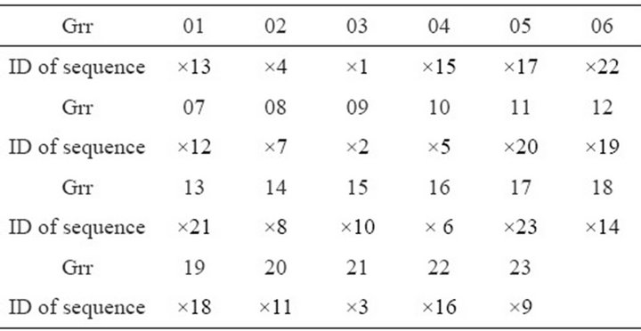
Table 6. New grey-relation rank (Grr) for No.1-23 of frogs.
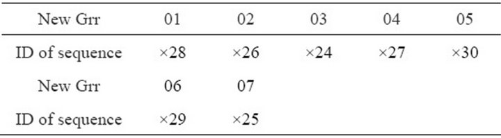
Table 7. New Grey-relation rank (Grr) for No.24-30 of frogs.
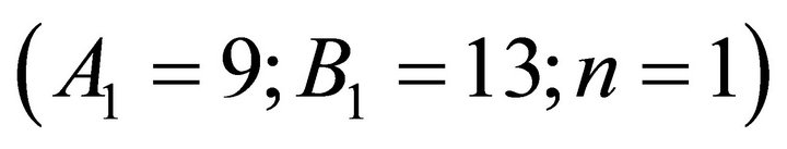
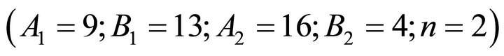
prove the accuracy of BPNN. To achieve this objective, the 5 neurons of the Frog ID with worse grey-relational rank was substituted for that with better rank (Tables 6 and 7) before BPNN analysis. For example, the 5 neurons of Frog ID 9 (Rank 23) should be substituted with those of Frog ID 13 (Rank 1) if we intended to exchange one set of neurons. Moreover, the neurons of Frog ID 9 (Rank 23) and Frog ID 16 (Rank 22) should be substituted with those of Frog ID 13 (Rank 1) and Frog ID 4 (Rank 2) if we intended to exchange two set of sequences.
The following tests were designed to collect further materials to investigate whether the grey-relational analysis can improve the accuracy of BPNN.
A. training stage (Network Structure is 4-3-1)
Test 1: Substitute  with
with 
Test 2: Substitute  with
with 
Test 3: Substitute  with
with 
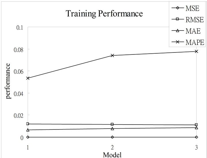
Figure 4. Comparisons of model 1 - model 3 in the training stage.
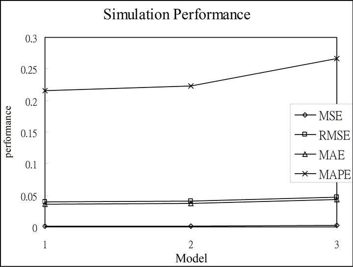
Figure 5. Comparisons of models 1 - 3 in the testing stage.

B. testing stage (Network Structure is 4-3-1)
Test 4: Substitute  with
with 

Test 5: Substitute  with
with 
C. testing stage (Network Structure is 4-5-1)
Test 6: Substitute  with
with 

Test 7: Substitute  with
with 

D. testing stage (Network Structure is 4-10-1)
Test 8: Substitute  with
with 
Test 9: Substitute  with
with 
For tests 1-3, the performance of network in the training and testing stages are shown in Tables 10 and 11. Tables 10 and 11 showed that the application of greyrelational analysis before the BPNN do not improve the BPNN network performance for both the training and testing stages.
For tests 4-9, the performance of network in the testing stage is shown in Table 12 and Figures 6-8. Table 12 and Figures 6-8 showed that the application of greyrelational analysis before the BPNN analysis does im-
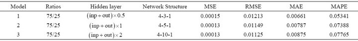
Table 8. The performance of network in the training stage.
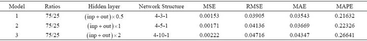
Table 9. The performance of network in testing stage.
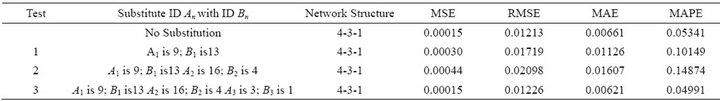
Table 10. The performance of network in the training stage.
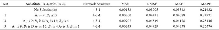
Table 11. The performance of network in the testing stage.
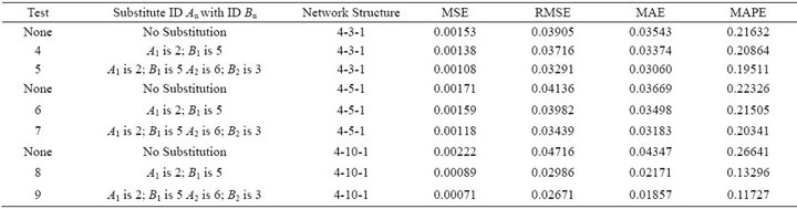
Table 12. The performance of network in testing stage.
prove the BPNN network performance. For example, for network structure 4-3-1 (see Table 12), it can be seen that the original computed values of MSE, RMSE, MAE and MAPE of BPNN (see No Substitution) is 0.00153, 0.03905, 0.03543 and 0.21632. If we substituted Frog ID 2 with Frog ID 5 (see Test 4 in Table 12), it can be seen that all the above computed values has declined. Moreover, if we substituted frogs ID 2 and ID 6 with frogs ID 5 and ID 3 (see Test 5 in Table 12), the above analysis yielded much more smaller values of MSE (0.00108), RMSE (0.03291), MAE (0.03060) and MAPE (0.19511). We can see that network structures 4-5-1 (Table 12 and Figure 7) and 4-10-1 (Table 12 and Figure 8) have exactly the same trend as network structure 4-3-1 (Table 12 and Figure 6).
The above results showed that the grey-relational analysis does not improve the of BPNN models in the training stage, but it does improve the results of BPNN models in the testing stage. It is reasonable to believe that the grey-relational analysis can improve the performance of BPNN. However, the above results of BPNN in the training stage should be further investigated to obtain more information to understand the above phenomenon.
Figure 9 shows the climbing abilities of frogs in the training stage obtained from BPNN and experiment for model 1. It can be seen that the numerical results have shown good agreement with experimental results. Figure 10 shows the climbing abilities of frogs in the testing stage obtained from BPNN and experiment for model 1. Again, it can be found that the numerical results have shown reasonable agreement with experimental results.
6. CONCLUSIONS
In this study, we apply Grey system theory and the Back-propagation neural network (BPNN) to investigate
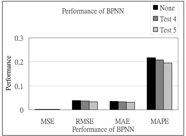
Figure 6. Comparison of test 4 and test 5 (Network Structure 4-3-1).
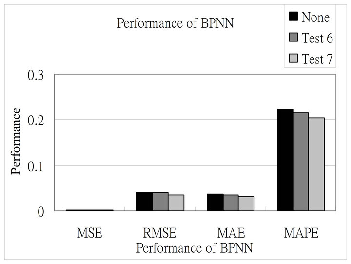
Figure 7. Comparison of test 6 and test 7(Network Structure 4-5-1).
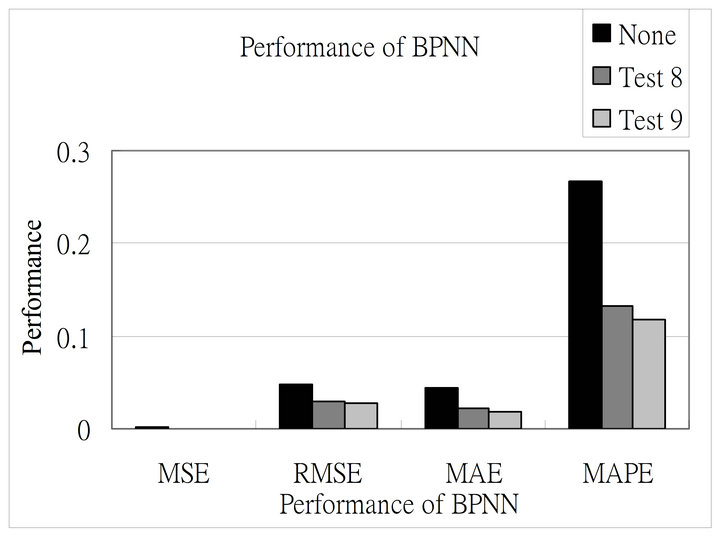
Figure 8. Comparison of test 8 and test 9 (Network Structure 4-10-1).
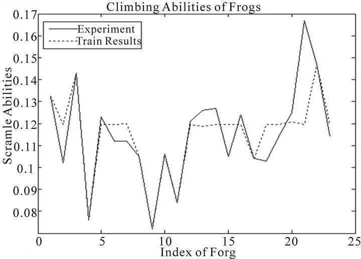
Figure 9. Comparison of the climbing abilities in the training stage from BPNN and experiment for model 1.
the climbing behavior of Buergeria robusta. Besides, grey-relational analysis and BPNN models with different
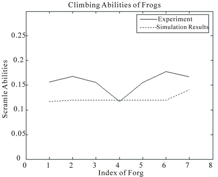
Figure 10. Comparisons of the climbing abilities in the testing stage from BPNN and experiment for model 1.
number of neurons in the hidden layer of samples are adopted. The results showed that the grey-relational analysis can be used to improve the simulation results of BPNN models.
In addition, BPNN models can be used to predict the climbing ability of Buergeria robusta with the input physical characteristics. The results obtained from this study can improve the communication and understanding of engineers and ecological researchers. In addition, they can provide further useful materials for engineers involved in future ecological engineering designs of banks throughout the world.
![]()
![]()
REFERENCES
- Yang, Y.R. (1998) A field guide to the frogs and toads of Taiwan, Nature and Ecology Photographer’s Society. Taipei.
- David and Markus (2012) Endemic species in Taiwan. The Global Biodiversity Information Facility (GBIF). http://ecat-dev.gbif.org/checklist/1055
- Bergen, S.D., Bolton, S.M. and Fridley, J.L. (2001) Design principles for ecological engineering. Ecological Engineering, 18, 201-210. doi:10.1016/S0925-8574(01)00078-7
- Mitsch, W.J. (1996) Ecological engineering: A new paradigm for engineers and ecologists, In: Schulze, P.C., Ed., Engineering within Ecological Constraints, National Academy Press, Washington DC, 114-132.
- Kim, K.C. and Byrne, L.B. (2006) Biodiversity loss and the taxonomic bottleneck: Emerging biodiversity science. Ecological Research, 21, 794-810. doi:10.1007/s11284-006-0035-7
- Stenseth, N.C., Mysterud, A., Ottersen, G., Hurrel, J.W., Chan, K.S. and Lima, M. (2002) Ecological effects of climate fluctuations. Science, 297, 1292-1296. doi:10.1126/science.1071281
- Dirzo, R. and Raven, P.H. (2003) Global state of biodiversity and loss. Annual Review of Environment and Resources, 28, 137-167. doi:10.1146/annurev.energy.28.050302.105532
- Turner, W.R., Nakamura, T. and Dinetti, M. (2004) Global urbanization and the separation of humans from nature. Bioscience, 54, 585-590. doi:10.1641/0006-3568(2004)054[0585:GUATSO]2.0.CO;2
- Biesmeijer, J.C., Roberts, S.P.M., Reemer, M., Ohlemiller, R., Edwards, M., Peeters, T., Schaffer, A.D., Potts, S.G., Keenkers, R., Thomas, C.D., Settele, J. and Kumin, W.E. (2006) Parallel declines in pollinators and insect-pollinated plants in Britain and the Netherlands. Science, 313, 351- 354. doi:10.1126/science.1127863
- Stuart, S.N., Chanson, J.S., Cox, N.A., Young, B.E., Rodrigues, A.S.L., Fischman, D.L. and Waller, R.W. (2004) Status and trends of amphibian declines and extinctions worldwide. Science, 306, 1783-1786. doi:10.1126/science.1103538
- Barinaga, M. (1990) Where have all the froggies gone? Science, 247, 1033-1034. doi:10.1126/science.247.4946.1033
- Blaustein, A.R. and Wake, D.B. (1990) Declining amphibian populations: A global phenomenon? Trends in Ecology and Evolution, 5, 203-204. doi:10.1016/0169-5347(90)90129-2
- Wake, D.B. (1991) Declining amphibian populations. Science, 253, 860.
- Woodford, J.E. and Meyer, M.W. (2003) Impact of lakeshore development on green frog abundance. Biological Conservation, 110, 277-284.
- Fujioka, M. and Lane, S.J. (1997) The impact of changing irrigation practices in rice fields on frog populations of the Kanto Plain, central Japan. Ecological Research, 12, 101-108. doi:10.1007/BF02523615
- Blaustein, A.R., Hoffman, P.D., Hokit, D.G., Kiesecker, J.M., Watts, S.C. and Havs, J.B. (1994) UV repair and resistance to solar UV-B in amphibian eggs: A link to population declines? Proceedings of the National Academy of Science, 91, 1791-1795. doi:10.1073/pnas.91.5.1791
- Pechmann, J.H.K., Scott, D.E., Semtitsch, R.D., Caldwell, J.P., Vitt, L.J. and Gibbsons J.W. (1991) Declining amphibian populations: The problem of separating human impacts from natural fluctuations. Science, 253, 892-895. doi:10.1126/science.253.5022.892
- Philips, K. (1990) Where have all the frogs and toads gone? BioScience, 40, 422-424. doi:10.2307/1311385
- Laurance, W.F. (1996) Catastrophic declines of Australian rainforest frogs is unusual weather responsible. Biological Conservation, 77, 203-212. doi:10.1016/0006-3207(95)00142-5
- Hamer, A.J., Lane, S.J. and Mahony, M.J. (2002) Management of freshwaterwetlands for the endangered green and golden bell frog (Litoria aurea): Roles of habitat determinants and space. Biological Conservation, 106, 413- 424. doi:10.1016/S0006-3207(02)00040-X
- Blaustein, A.R., Wake, D.B. and Sousa, W.P. (1994) Amphibian declines: Judging stability, persistence, and susceptibility of populations to local and global extinctions. Conservation Biology, 8, 60-71. doi:10.1046/j.1523-1739.1994.08010060.x
- Gillespie, G.R. (2002) Impacts of sediment loads, tadpole density, and food type on the growth and development of tadpoles of the spotted tree frog. Biological Conservation, 106, 141-150. doi:10.1016/S0006-3207(01)00127-6
- Lue, K.Y. (1996) A handbook of amphibian animal resources. Council of Agriculture, Executive Yuan, 31-33.
- Chen, W.S. (2003) 31 frogs in Taiwan. Wild Bird Society of Taipei, 62-63.
- Hou, W.S., Chang, Y.H. and Wang, H.W. (2008) Climatic effects and impacts of lakeshore bank designs on the activity of Chirixalus idiootocus in Yilan, Taiwan. Ecological Engineering, 32, 52-59. doi:10.1016/j.ecoleng.2007.09.004
- Hou, W.S., Chang, Y.H., Chuang, T.F. and Chen, C.H. (2010) Effect of ecological engineering design on biological motility and habitat environment of hynobius arisanensis at high altitude areas in Taiwan. Ecological Engineering, 36, 791-798. doi:10.1016/j.ecoleng.2010.02.004
- Chang, Y.H., Wang, H.W. and Hou, W.S. (2011) Effects of construction materials and design of lake and stream banks on climbing ability of frogs and salamanders. Ecological Engineering, 37, 1726-1733. doi:10.1016/j.ecoleng.2011.07.005
- Deng, J.L. (1989) Introduction to grey system. The Journal of Grey System, 1, 1-24.
- Yu, W.C. (1976) Biometrics with experiment designs. Nung-Ying Books, taipei, 234-262.
- Green, D.M. (1981) Adhesion and toe-pads of tree frogs. Copeia, 4, 790-796. doi:10.2307/1444179
- Lin, S.T., Horng, S.H, Lee, B.H., Fan, P., Pan, Y., Lai, J.L., Chen, R.J. and Khan, M.K. (2011) Application of grey-relational analysis to find the most suitable watermarking scheme. International Journal of Innovative Computing, Information and Control, 7, 5389-5401.
- Waller, B. and Aiken, M. (1998) Predicting prepayment of residential mortgages: A neural network approach, International Journal of Information and Management Sciences, 9, 37-44.
- Jost, A. (1993) Neural networks: A logical progression in credit and marketing decision system, Credit World, 81, 26-33.
- Yang, H.C. and Chang, F.J. (2005) Modeling the combined open channel flow by artificial neural network. Hydrological Processes, 19, 3747-3762. doi:10.1002/hyp.5858
- Han, M. and Xi, J. (2004) Efficient clustering of radial basis perception neural network for pattern recognition. Pattern Recognition, 37, 2059-2067.
- Burger, C.J.S.C., Dohnal, M., Kathrada, M. and Law, R. (2001) A practitioners guide to time-series method for tourism demand forecasting—A case study of Durban, South Africa. Tourism Management, 22, 403-409. doi:10.1016/S0261-5177(00)00068-6
- Schollhom, W.I. (2004) Applications of artificial neural nets in clinical biomechanics. Clinical Biomechanics, 19, 876-898. doi:10.1016/j.clinbiomech.2004.04.005
- Buscb, A.C., Schefl’er, C. and Basson, A.H., (2009) Development and testing of a prototype reflex measurement system employing artificial neural networks. Computer Methods and Programs in Biomedicine, 94, 15-25. doi:10.1016/j.cmpb.2008.08.008
- Barton, G., Lisboa, P., Lees, A. and Attficld, S. (2007) Gait quality assessment using self-organising artificial neural networks, Gait & Posture, 25, 374-379. doi:10.1016/j.gaitpost.2006.05.003
- Wu, D., Yang, Z. and Liang, L. (2006) Using DEA-neural network approach to evaluate a branch efficiency of a large Canadian bank. Expert System with Applications, 32, 108-115. doi:10.1016/j.eswa.2005.09.034
- MATLAB (2011) Getting started guide. The MathWorks, Inc, Natick.
- Tsou, K.W., Chang, Y.S. and Tu, C.H. (2006) A forecast of building destruction in earthquakes: Applications of artificial neural network, Journal of Housing Studies, 15, 21-42.