Open Journal of Statistics
Vol.1 No.2(2011), Article ID:6549,13 pages DOI:10.4236/ojs.2011.12005
Estimation Using Censored Data from Exponentiated Burr Type XII Population
Department of Mathematics, Alexandria University, Egypt
E-mail: dr_essak@hotmail.com
Received May 3, 2011; revised May 25, 2011; accepted June 2, 2011
Keywords: Exponentiated distribution, Proportional reversed hazard rate model, Lehmann alternatives, Maximum likelihood and Bayes estimation, Burr type XII distribution, subjective prior, SE and LINEX loss functions, MCMC
Abstract
Maximum likelihood and Bayes estimators of the parameters, survival function (SF) and hazard rate function (HRF) are obtained for the three-parameter exponentiated Burr type XII distribution when sample is available from type II censored scheme. Bayes estimators have been developed using the standard Bayes and MCMC methods under square error and LINEX loss functions, using informative type of priors for the parameters. Simulation comparison of various estimation methods is made when n = 20, 40, 60 and censored data. The Bayes estimates are found to be, generally, better than the maximum likelihood estimates against the proposed prior, in the sense of having smaller mean square errors. This is found to be true whether the data are complete or censored. Estimates improve by increasing sample size. Analysis is also carried out for real life data.
1. Introduction
Analogous to the Pearson system of distributions, Burr [1] introduced a system that includes twelve types of cumulative distribution functions (CDF) which yield a variety of density shapes. This system is obtained by considering CDF’s satisfying a differential equation which has a solution, given by:

where  is chosen such that
  is a CDF on the real line. Twelve choices for
 , made by Burr, resulted in twelve distributions from which types III, X and XII have been frequently used. The flexibilities of Burr XII distribution were investigated by Hatke [2], Burr [3], Rodrigues [4] and Tadikamalla [5].
In a different direction, it was Takahasi[6] who first noticed that the 3-parameter Burr XII probability density function (PDF) can be obtained by compounding a Weibull PDF with a gamma PDF. That is, if X|θ~ Weibull (θ, β) and θ~ gamma (γ, δ) then the compound PDF, say g(x|β, γ, δ), is given by

which is the 3-parameter Burr XII (β, γ, δ) PDF.
If δ = 1, this PDF reduces to the 2-parameter Burr XII (β, g), whose PDF, CDF, SF, and HRF are given, for x > 0, (β, g > 0), by:
 (1.1)
(1.1)
 (1.2)
(1.2)
 (1.3)
(1.3)
 .(1.4)
The Burr XII and its reciprocal Burr III distributions have been used in many applications such as actuarial science, as in Embrechts et al. [7] and Klugman[8], quantal bioassay as in Drane et al. [9], economics, as in McDonald and Richards [10], Morrison and Schmittlein [11], Schmittlein [12], McDonald [13], forestry,as in Lindsay et al. [14], exotoxicology, as in Shao [15], life testing and reliability, as in Dubey [16,17], Papadopoulos [18], Lewis [19], Evans and Ragab [20], Lingappaiah [21], Jaheen [22], AL-Hussaini et al. [23], Shah and Gokhale [24], AL-Hussaini and Jaheen, [25,26] and Moore and Papadopoulos [27], among others. Khan and Khan [28] and AL-Hussaini [29] characterized the Burr XII distribution. Lewis [19] proposed the use of the Burr XII distribution as a model in accelerated life test data representing times to break down of an insulating fluid. Constant partially accelerated life tests for Burr XII distribution with progressive type II censoring was investigated by Abdel-Hamid [30]. Prediction of future observables from Burr XII distribution was studied by Nigm [31], AL-Hussaini and Jaheen [32,33], AL-Hussaini [34] and AL-Hussaini and Ahmad [35], among others. The extended 3-parameter Burr XII was applied in flood frequency analysis by Shao et al. [36].
Adding one or more parameters to a distribution makes it richer and more flexible for modeling data. There are different ways for adding parameter(s) to a distribution. Marshall and Olkin [37] added one positive parameter to a given (general) SF. AL-Hussaini and Ghitany [38] added two parameters (r, p) to a SF by considering a countable mixture of positive integer powers of general SFs in which the mixing proportions are Pascal (r, p). A new family of distributions as a countable mixture with Poisson added parameters was obtained by AL-Hussaini and Gharib [39].
Adding a parameter by exponentiation goes back to Verhulst [40], who raised his 1838 logistic CDF (see [41]) to a positive power. Ahuja and Nash [42] seemed to have been the first to raise Verhulst [43] exponential CDF to a positive power.
AL-Hussaini [44] made some preliminary studies for properties of exponentiated class of distributions of the form
 (1.5)
(1.5)
where G(x) may depend on a vector of parameters .
.
Inference (estimation and prediction) based on censored samples from exponentiated populations with CDF of the form (1.5) was made by AL-Hussaini [45] who also reviewed the applications of exponentiated Weibull and exponentiated exponential families. (See pages 2 and 3 in the introduction of AL-Hussaini [45] and the references therein).
Exponentiated distributions are also known as proportional reversed hazard rate models (PRHRM) with constant of proportionality α. Reversed hazard rate function (RHRF) is defined by
 .
.
If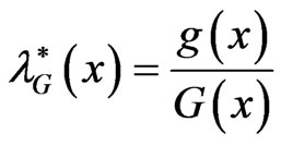 , where
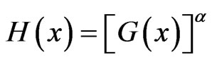 , then
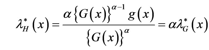 .
.
That is,  is proportional to
  with constant of proportionality
 . This is why the exponentiated distribution
  is called PRHRM. See Gupta and Gupta [46]. Exponentiated distributions are also known as Lehmann alternatives, due to Lehmann [47], who defined the model, when
  is a positive integer, as a non-parametric class of alternatives.
In general, the PDF, SF and HRF of the exponentiated CDF (1.5) are given by:
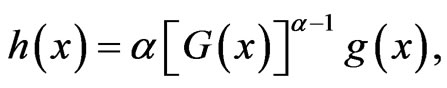 (1.6)
(1.6)
 (1.7)
(1.7)
 (1.8)
(1.8)
Relation between the HRF  of H and the HRF
  of G
of G
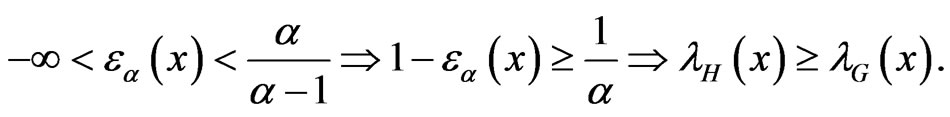
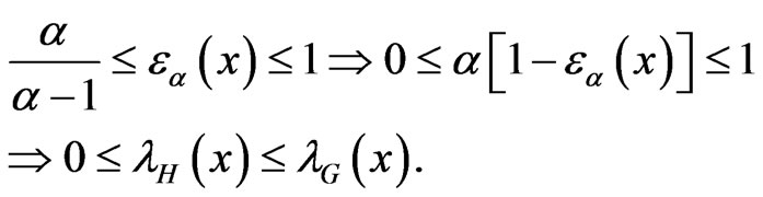
If 0 < α < 1, then  for all x and if
  then
then , for all x. This follows by observing that
 (1.9)
(1.9)
where
 .(1.10)
If , then
If , then
Notice that, for ,
,  ,
,  by using L’Hopital’s rule. It is clear, from (1.9), that
  is not proportional to
It can be shown that the CDF  is related to the HRF
  and RHRF
  by the relation
 .(1.11)
2. Estimation of Parameters, SF and HRF
Suppose that n items, whose life times follow a CDF , where the CDF G(x) may depend on a vector of parameters
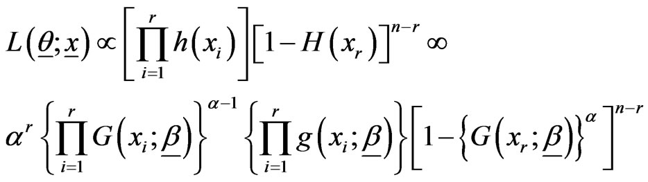
 , are put on test and that the test is terminated at the rth failure (type II censoring). Suppose that the life times of the first r failed items
  have been observed. The likelihood function (LF) is then given by
 ,(2.1)
where h(·)and  are the PDF and SF corresponding to H(·),
  and
and . In the EBurr XII (α, β, γ), the CDF G(·) is Burr XII (β, γ), given by (1.2), where
 .
.
2.1. All Parameters of H Are Unknown
In this section, we consider the case in which the CDF G(·) is Burr XII , where
  and all parameters of H are unknown. In this case we have a vector of unknown parameters
  of H.
of H.
2.1.1. Maximum Likelihood Estimation
The LF is given, in terms of G(x) and g(x), as:
 (2.2)
(2.2)
The log-LF is then given by
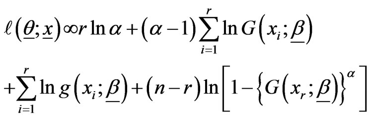 (2.3)
(2.3)
Differentiate (2.3) partially with respect to α and  and then equate to zero, to get
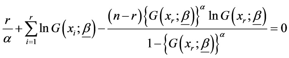 ,(2.4)
 , (2.5)
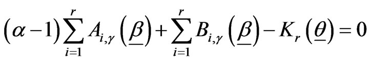 ,(2.6)
where
 ,
,
 ,
,
 ,
,
 and
and .
.
The ML estimator of a can be written, using (2.4) and (2.5), in terms of , as
, as
 .(2.7)
The MLEs of  and
and , say
, say  and
and  can be obtained by maximizing the log-likelihood function with respect to
  and
and . Once
  and
and  are obtained, the ML estimator of
 , say
, say , can be obtained from (2.7).
The MLEs are used in determining the vector of hyper-parameters in the Bayes case (see section 4).
2.1.2. Standard Bayes Method
We assume that α is independent of (β, γ) and that ,
,  and
and  so that the prior PDF of
  is given by
 ,
,

 .
.
LF (2.2) can be rewritten in the form
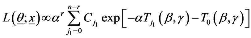 ,(2.8)
where,
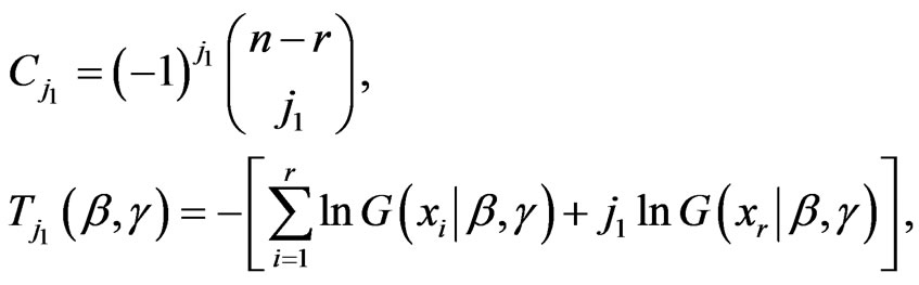 (2.9)
(2.9)
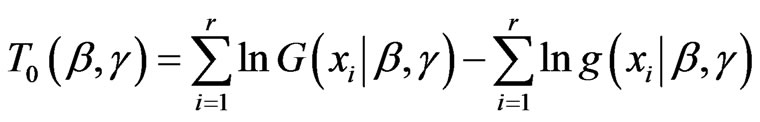 .(2.10)
The posterior PDF is then given, from LF (2.8) and the prior  by
by
 .(2.11)
where
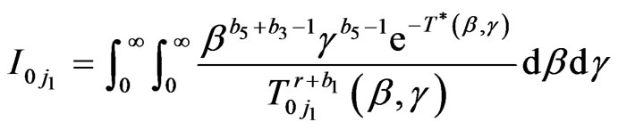 ,
,
 (2.12)
 and
and  are given by (2.9) and (2.10).
2.1.2.1. Bayes Estimators under SEL Function
AL-Hussaini [45] showed that, under squared error loss, the Bayes estimators of 
 and
and  are given, for any G (which has parameters
  and
and ), by
), by
 (2.13)
 (2.14)
where
 ,
, 
 ,
,
 ,
,
 ,
,
 .
.
 ,
,
 ,
,
 .
.
2.1.2.2. Bayes estimators under LINEX loss Function
The SEL function has probably been the most popular loss function used in literature. The symmetric nature of SEL function gives equal weight to overand underestimation of the parameters under consideration. However, in life testing, over estimation may be more serious than under estimation or vice versa. Research has been directed towards asymmetric loss functions. Varian [48] suggested the use of linear-exponential (LINEX) loss function to be of the form
 ,(2.15)
where  and
and .
.
Thompson and Basu [49] generalized the LINEX loss function to the squared-exponential (SQUAREX) loss function to be of the form
 where
where  and
and  are as before.
The SQUAREX loss function reduces to the LINEX loss function if . If
. If , the SQUAREX loss function reduces to the SEL function.
In this paper, we shall use the LINEX loss function, as the SQUAREX loss function could be similarly treated. Using the LINEX loss function, the Bayes estimator of , a function of the (vector) of parameter(s)
 , is given by
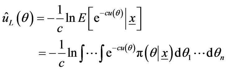 ,(2.16)
where  is the posterior PDF of the vector of parameters
 , given the set of data
 . In general, the integrals are taken over the n-dimensional space
 .
.
2.2. Theorem
The Bayes estimators of α, â, g,  and
and  under LINEX loss are
 (2.17)
where
 (2.18)
 (2.19)
 is given in (2.9),
 (2.20)
 (2.21)
The proof is given in the Appendix 1.
3. Numerical Results and Comparisons
The estimates of α, â, g,  and
and  and their mean square errors (MSE) are computed by using the MLE, standard Bayes method (SB) and MCMC algorithm (SEL and LINEX loss). Such an algorithm is given in Appendix 2.
To see the effect of sample size on the performance of ML and Bayes estimates, a comparison of different estimation methods is made when 1000 samples of size n = 20, 40, 60 each, are drawn from the population distribution, in the complete sample case and when data are censored at the 10% and 25% levels, for each sample size.
Under the LINEX loss, different values of c (−0.5, 0.01, 0.1) are used, for different sample sizes and censoring values. The computational values are reported in Tables 1(a)-(c).
The actual population values are α = 2.5, β = 1.5, γ = 2. The hyper-parameters are b1 = 0.6, b2 = 0.6, b3 = 2, b4 = 3, b5 = 2. It may be noticed that with the values of α = 2.5, β = 1.5, γ = 2 the values given for  are the averages over the 1000 samples. For
 , the actual values for
  and
and  are respectively 0.719 and 1.024.
3.1. Remark
It can be numerically shown that the vector of parameters  satisfying the log-likelihood equations (2.4)-(2.6) actually maximizes the likelihood function (2.3). This is done by applying Theorem (7-9) on p. 152 of Apostol [50].
3.2. Simulation Comparisons
Simulation comparisons of various estimation methods is made when n = 20, 40, 60 and censored data. From Tables 1(a-c), below, it may be observed that the Bayes estimates are, generally, better than the MLEs against the proposed prior in the sense of having smaller MSEs. Even for sample size as small as n = 20, good Bayes estimates (with smaller MSEs), are obtained under the LINEX loss function as well as SEL with the same censoring level. All estimates improve by increasing sample size. Analysis is also carried out for real life data, in Section 4.
4. Real Life Data
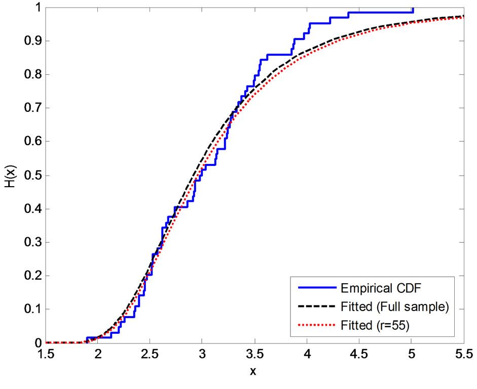
In this section we analyze real life data set to demonstrate how the proposed methods can be used in practice. To check the validity of the fitted model, we use Kolmogorov-Smirnov goodness of fit test (KS) to test “the fitted distribution function is H(x)”. We plot the fitted distribution function H(x) using the three methods (ML, SBM, MCMC) and the empirical distribution function in each case.
The breaking strengths of 64 (= n) single carbon fibers of length 10 (Lawless [51],p. 573) are :
1.901, 2.132, 2.203, 2.228, 2.257, 2.350, 2.361, 2.396, 2.397, 2.445, 2.454, 2.454, 2.474, 2.518, 2.522, 2.525, 2.532, 2.575, 2.614, 2.616, 2.618, 2.624, 2.659, 2.675,

Table 1. (a) Complete sample (r = 20); (b) Censored sample (r = 18); (c) Censored sample (r = 15).
2.738, 2.740, 2.856, 2.917, 2.928, 2.937, 2.937, 2.977, 2.996, 3.030, 3.125, 3.139, 3.145, 3.220, 3.223, 3.235, 3.243, 3.264, 3.272, 3.294, 3.332, 3.346, 3.377, 3.408, 3.435, 3.493, 3.501, 3.537, 3.554, 3.562, 3.628, 3.852, 3.871, 3.886, 3.971, 4.024, 4.027, 4.225, 4.395, 5.020.
In the complete sample case (r = n), the estimates of the parameters, SF, HRF at  and the corresponding p-value of KS goodness of fit test are given in Table 2(a). The Bayes estimates (SB and MCMC) are calculated for the hyper-parameters b1 = 180, b2 = 0.6, b3 = 2, b4 = 3, b5 = 2. We have used the same values of
  as in the simulation study. To give a value for
 , we noticed that MLE of α is quite large. In the Bayes case, the mean of the gamma (
 ) prior depends on
 . For fixed
  at 0.6, this mean is large if
  is large. After some fitting trials we found that
  gives a good fit. See Figure 1.
Suppose that, this test is terminated after the first 55 (= r) failures, the estimates of the parameters, SF, HRF at  and the corresponding p value of KolmogorovSmirnov goodness of fit test (KS) are given in Table 2(b).
5. Concluding Remarks
Estimation of the parameters, survival and hazard rate functions are obtained when data are drawn from the three-parameter exponentiated Burr type XII distribution. Type II censoring is imposed on data. The maximum likelihood and Bayes methods are used in estimation. In the Bayes case, the estimators are obtained under squared-error and LINEX loss functions. The methods are compared by computing the mean squared errors (overall Bayes risks, in the Bayes case).
Kolmogorov-Smirnov goodness of fit test shows that the exponentiated Burr type XII distribution fits the data of the breaking strengths of 64 (=n) single carbon fibers of length 10, given in Lawless, in all cases.
From Tables 1(a)-(c), it may be noticed that the Bayes estimates are, generally, better than the MLEs against the
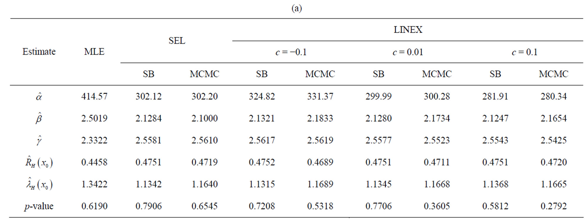

Table 2. (a) Complete Sample (r = 64); (b) Censored Sample (r = 55).
 (a)
(a)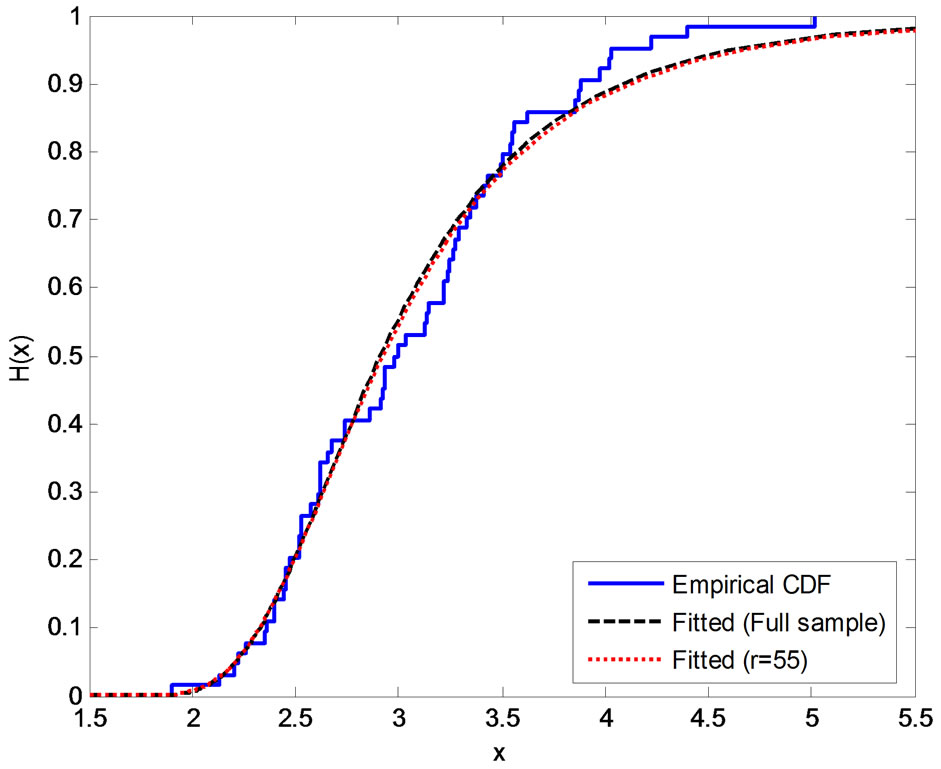 (b)
(b)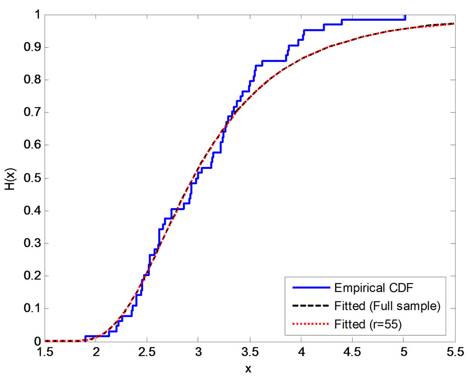 (c)
(c)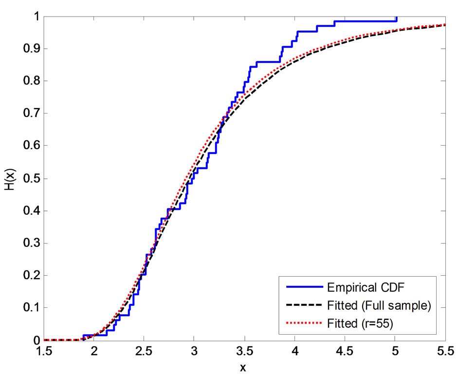 (d)
(d)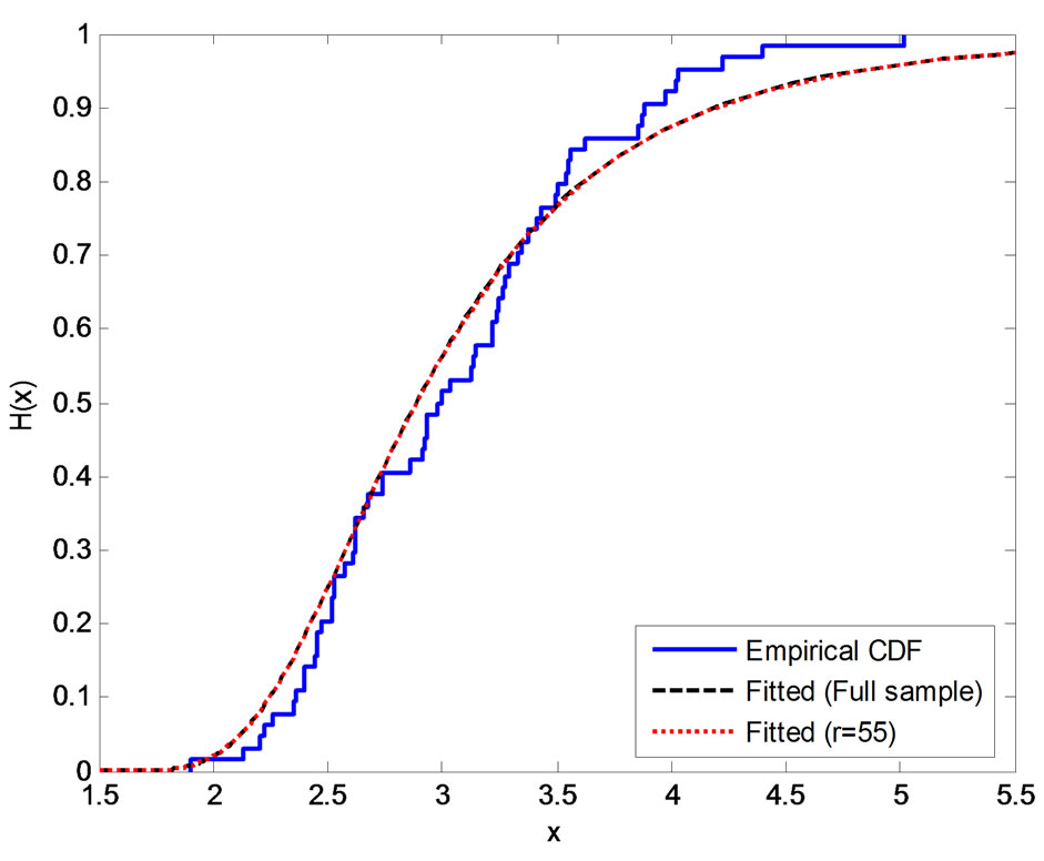 (e)
(e)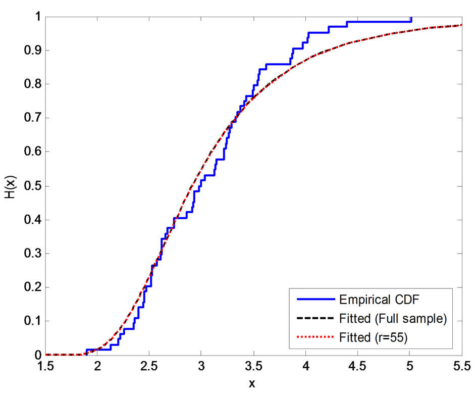 (f)
(f)
Figure 1. Empirical and fitted CDF using different methods of estimation, (a) MLE; (b) SEL (SB); (c) SEL (MCMC); (d) LINEX (SB), c = −0.1; (e) LINEX (SB), c = 0.01; (f) LINEX (SB), c = 0.1.
proposed prior in the sense of having smaller MSEs. Even for sample size as small as n = 20, good Bayes estimates (with smaller MSEs), are obtained under LINEX loss function as well as SEL with the same censoring level. All estimates improve by increasing sample size.
6. References
[1] I. W. Burr, “Cumulative Frequency Functions,” The Annals of Mathematical Statistics, Vol. 1, No. 2, 1942, pp. 215-232. doi:10.1214/aoms/1177731607
[2] M. A. Hatke, “A Certain Cumulative Probability Function,” The Annals of Mathematical Statistics, Vol. 20, No. 3, 1949, pp. 461-463. doi:10.1214/aoms/1177730002
[3] I. W. Burr, “Parameters for a General System of Distributions to Match a Grid of α3 and α4,” Communications in Statistics-Theory and Methods, Vol. 2, No. 2, 1973, pp. 1-21. doi:10.1080/03610927308827052
[4] R. N. Rodriguez, “A Guide to the Burr Type XII Distributions,” Biometrika, Vol. 64, No. 1, 1977, pp. 129-134. doi:10.1093/biomet/64.1.129
[5] P. R. Tadikamalla, “A Look at the Burr and Related Distributions,” International Statistical Review, Vol. 48, No. 3, 1980, pp. 337-344. doi:10.2307/1402945
[6] K. Takahasi, “Note on the Multivariate Burr’s Distribution,” Annals of the Institute of Statistical Mathematics, Vol. 17, No. 1, 1965, pp. 257-260. doi:10.1007/BF02868169
[7] P. Embrechts, C. Kluppelberg and T. Mikosch, “Modeling Extremal Events,” Springer-Verlag, Berlin, 1977.
[8] A. S. Klugman, “Loss Distributions,” Wiley Interscience, New York, 1986, pp. 31-55.
[9] S. W. Drane, D. B. Owen and G. B. Seibetr Jr., “The Burr Distribution and Quantal Responses,” Statistical Papers, Vol. 19, No. 3, 1978, pp. 204-210. doi:10.1007/BF02932803
[10] J. B. McDonald and D. O. Richards, “Model Selection: Some Generalized Distributions,” Communications in Statistics-Theory and Methods, Vol. 17, 1978, pp. 287-296.
[11] D. G. Morrison and D. C. Schmittlein, “Jobs, Strikes and Wars: Probability Models for Duration,” Organizational Behavior and Human Performance, Vol. 25, No. 2, 1980, pp. 224-251. doi:10.1016/0030-5073(80)90065-3
[12] D. C. Schmittlein, “Some Sampling Properties of a Model for Income Distribution,” Journal of Business and Economic Statistics, Vol. 1, No. 2, 1983, pp. 147-153. doi:10.2307/1391855
[13] J. B. McDonald, “Some Generalized Function for the Size Distribution of Income,” Econometrica, Vol. 52, No. 3, 1984, pp. 647-663. doi:10.2307/1913469
[14] S. R. Lindsay, G. R. Wood and R. C. Woollons, “Modeling the Diameter Distribution of Forest Stands Using the Burr Distribution,” Journal of Applied Statistics, Vol. 23, No. 6, 1996, pp. 609-619. doi:10.1080/02664769623973
[15] Q. Shoa, “Estimation for Hazardous Concentrations Based on NOEC Toxicity Data: An Alternative Approach,” Environmetrics, Vol. 11, No. 5, 2000, pp. 583-595. doi:10.1002/1099-095X(200009/10)11:5<583::AID-ENV456>3.0.CO;2-X
[16] S. D. Dubey, “Statistical Contributions to Reliability Engineerings,” Aerospace Research Laboratories, Charlottesville, 1972.
[17] S. D. Dubey, “Statistical Treatment of Certain Life Testing and Reliability Problems,” Aerospace Research Laboratories, Charlottesville, 1973.
[18] A. S. Papadopoulos, “The Burr Distribution as a Life Time Model from a Bayesian Approach,” IEEE Transactions on Reliability, Vol. 27, No. 5, 1978, pp. 369-371. doi:10.1109/TR.1978.5220427
[19] A. W. Lewis, “The Burr Distribution as a General Parametric Family in Survivor-Ship and Reliability Theory Applications,” Ph.D. Thesis, University of North Carolina, North Carolina, 1981.
[20] I. G. Evans and A. S. Ragab, “Bayesian Inferences Given a Type-2 Censored Sample from Burr Distribution,” Communications in Statistics-Theory and Methods, Vol. 12, No. 13, 1983, pp. 1569-1580. doi:10.1080/03610928308828551
[21] G. S. Lingappaiah, “Bayesian Approach to the Estimation of Parameters in the Burr’s XII Distribution with Outliers,” Journal of Orissa Mathematical Society, Vol. 1, 1983, pp. 55-59.
[22] Z. F. Jaheen, “Bayesian Estimations and Predictions Based on Single Burr type XII Models and Their Finite Mixture,” Ph.D. Thesis, University of Assiut, Assiut, 1993.
[23] E. K. AL-Hussaini, M. A. Mousa and Z. F. Jaheen, “Estimation under the Burr Type XII Failure Model: A Comparative Study,” Test, Vol. 1, No. 1, 1992, pp. 33-42.
[24] A. Shah and D. V. Gokhale, “On Maximum Product of Spacings (MPS) Estimation for Burr XII Distribution,” Communications in Statistics-Theory and Methods, Vol. 22, 1993, pp. 615-641.
[25] E. K. AL-Hussaini and Z. F. Jaheen, “Bayes Estimation of the Parameters, Reliability and Failure Rate Functions of the Burr Type XII Failure Model,” Journal of Statistical Computation and Simulation, Vol. 41, No. 1-2, 1992, pp. 31-40. doi:10.1080/00949659208811389
[26] E. K. AL-Hussaini and Z. F. Jaheen, “Approximate Bayes Estimators Applied to the Burr Model,” Communications in Statistics-Theory and Methods, Vol. 23, No. 1, 1994, pp. 99-121.
[27] D. Moore and A. S. Papadopoulos, “The Burr Type XII Distribution as a Failure Model under Various Loss Functions,” Microelectronics Reliability, Vol. 40, No. 12, 2000, pp. 2117-2122. doi:10.1016/S0026-2714(00)00031-7
[28] A. H. Khan and A. I. Khan, “Moments of Order Statistics from Burr’s Distribution and Its Characterization,” Metron-International Journal of Statistics, Vol. 45, 1987, pp. 21-29.
[29] E. K. AL-Hussaini, “A Characterization of the Burr Type XII Distribution,” Applied Mathematics Letters, Vol. 4, No. 1, 1991, pp. 59-61. ![]() doi:10.1016/0893-9659(91)90123-D
doi:10.1016/0893-9659(91)90123-D
[30] A. H. Abdel-Hamid, “Constant-Partially Accelerated Life Tests for Burr XII Distribution with Progressive Type II Censoring,” Computational Statistics & Data Analysis, Vol. 53, No. 7, 2009, pp. 2511-2523. doi:10.1016/j.csda.2009.01.018
[31] A. M. Nigm, “Prediction Bounds for the Burr Model,” Communications in Statistics-Theory and Methods, Vol. 17, No. 1, 1988, pp. 287-296. doi:10.1080/03610928808829622
[32] E. K. AL-Hussaini and Z. F. Jaheen, “Bayes Prediction Bounds for the Burr Type XII Failure Model,” Communications in Statistics-Theory and Methods, Vol. 24, No. 7, 1995, pp. 1829-1842. doi:10.1080/03610929508831589
[33] E. K. AL-Hussaini and Z. F. Jaheen, “Bayesian Prediction Bounds for the Burr Type XII Distribution in the Presence of Outliers,” Journal of Statistical Planning and Inference, Vol. 55, No. 1, 1996, pp. 23-37. doi:10.1016/0378-3758(95)00184-0
[34] E. K. AL-Hussaini, “Bayesian Predictive Density of Order Statistics Based on Finite Mixture Models,” Journal of Statistical Planning and Inference, Vol. 113, No. 1, 2003, pp. 15-24. doi:10.1016/S0378-3758(01)00297-X
[35] E. K. AL-Hussaini and A. A. Ahmad, “On Bayesian Interval Prediction of Future Records,” Test, Vol. 12, No. 1, 2003, pp. 79-99. doi:10.1007/BF02595812
[36] Q. X. Shao, H. Wong, J. Xia, and W.-C. Ip, “Models for Extremes Using the Extended Three-Parameter Burr XII System with Application to Flood Frequency Analysis,” Hydrological Sciences, Vol. 49, No. 4, 2004, pp. 685-702.
[37] A. W. Marshall and I. Olkin, “A New Method for Adding a Parameter to a Family of Distributions with Applications to the Exponential and Weibull Families,” Biometrika, Vol. 84, No. 3, 1997, pp. 641-652. doi:10.1093/biomet/84.3.641
[38] E. K. AL-Hussaini and M. Ghitany, “On Certain Countable Mixtures of Absolutely Continuous Distributions,” Metron-International Journal of Statistics, Vol. 18, No. 1, 2005, pp. 39-53.
[39] E. K. AL-Hussaini and M. A. Gharib, “A New Family of Distributions as a Countable Mixture with Poisson Added Parameter,” Journal of Statistical Theory and Applications, Vol. 8, 2009, pp. 169-190.
[40] P. F. Verhulst, “Recheches Mathématiques sur la loi d’accroissement de la Population,” Nouveaux Mémoire de l’Academie Royale de Sciences et Belle-Lettres de Bruxelles, Vol. 18, 1845, pp. 1-42.
[41] P. F. Verhulst, “Notice sur la Loi que la Population Poursuit dans son Accroissement,” Correspondance Mathématique et physique, publiée par L.A.L. Quetelet, Vol. 10, 1838, pp. 113-121.
[42] J. C. Ahuja and S. W. Nash, “The Generalized GompertzVerhulst Family of Distributions,” Sankhyā, Vol. 29, No. 2, 1967, pp. 141-161.
[43] P. F. Verhulst, “Deuxié memémoire sur la loi d’accroissment de la Population,” Mémoire de l’Academie Royale de Sciences, des Lettreset de Beaux-Arts de Belgique, Series 2, Vol. 20, 1847, pp. 1-32.
[44] E. K. AL-Hussaini, “On Exponentiated Class of Distributions,” Journal of Statistical Theory and Applications, Vol. 9, 2010, pp. 41-63.
[45] E. K. AL-Hussaini, “Inference Based on Censored Samples from Exponentiated Populations,” Test, Vol. 19, No. 3, 2010, pp. 487-513. doi:10.1007/s11749-010-0183-5
[46] R. C. Gupta and R. D. Gupta, “Proportional Reversed Hazard Rate Model and Its Applications,” Journal of Statistical Planning and Inference, Vol. 137, No. 11, 2007, pp. 3525-3536. doi:10.1016/j.jspi.2007.03.029
[47] E. L. Lehmann, “The Power of Rank Tests,” The Annals of Mathematical Statistics, Vol. 24, No. 1, 1953, pp. 28-43. doi:10.1214/aoms/1177729080
[48] H. Varian, “A Bayesian Approach to Real Estate Assessment,” In: S. E. Fienberg and A. Zellner, Eds., Studies in Bayesian Econometrics and Statistics, North-Holland, Amsterdam, 1975, pp. 195-208.
[49] R. D. Thompson and A. P. Basu, “Asymmetric loss Function for Estimating System Reliability,” In: D. A. Berry, K. M. Chaloner and J. K. Geweke, Eds., Bayesian Analysis in Statistics and Econometrics, Wiley Series in Probability and Statistics, New York,1996.
[50] T. M. Apostol, “Mathematical Analysis,” 3rd Edition, Addison-Wesley, Boston, 1957.
[51] J. F. Lawless, “Statistical Models and Methods for Lifetime Data,” 2nd Edition, Wiley, New York, 2003.
[52] M. K. Cowles and B. P. Carlin, “Markov Chain Monte Carlo Convergence Diagnostics: A Comparative Review,” Journal of the American Statistical Association, Vol. 91, No. 434, 1996, pp. 883-904. doi:10.2307/2291683
[53] A. Gelman and D. B. Rubin, “Inference from Iterative Simulation Using Multiple Sequences,” Statistical Science, Vol. 7, No. 4, 1992, pp. 457-472. doi:10.1214/ss/1177011136
[54] G. O. Roberts, A. Gelman and W. R. Gilks, “Weak Convergence and Optimal Scaling of Random Walk Metropolis Algorithms,” The Annals of Applied Probability, Vol. 7, No. 1, 1997, pp. 110-120. doi:10.1214/aoap/1034625254
[55] L. Tierney, “Markov Chains for Exploring Posterior Distributions,” The Annals of Statistics, Vol. 22, No. 4, 1994, pp. 1701-1762. doi:10.1214/aos/1176325750
[56] D. Gamerman and H. P. Lopes, “Markov Chain Monte Carlo: Stochastic Simulation for Bayesian Inference,” 2nd Edition, Chapman and Hall, London, 2006.
[57] D. Sinha, T. Maiti, J. Ibrahim and B. Ouyang, “Current Methods for Recurrent Events Data with Dependent Termination: A Bayesian Perspective,” Journal of the American Statistical Association, Vol. 103, 2008, pp. 866-878. doi:10.1198/016214508000000201
Appendix 1
Proof of Theorem From (2.16) we have,
 .
.
Using the joint posterior , given by (2.8),

Similarly ,

and
and

 and
and are given by (2.18) and (2.19).
Appendix 2
Implementation of MCMC method To use the MCMC method in computing Bayes estimates of , at specific value of
 , we first notice that the general problem is in evaluating the integral
 , assuming that
 . If we can draw samples
 from
from , then Monte Carlo integration allows us to estimate this expectation by the average:
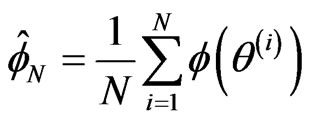 . If we generate samples using a Markov chain (aperiodic, irreducible and has a stationary distribution with PDF
 ), then by the ergodic theorem
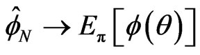 , as
, as . The estimate
  is called an ergodic average. Also for such chains, if the variance of
  is finite, the central limit theorem holds and convergence occurs geometrically. Early iterations
 , reflect starting value
 . These iterations are called burn-in. After the burn-in, we say that the chain has ‘converged’. The burn-in are omitted from the ergodic averages to end up with
 .
.
Methods for determining M are called convergence diagnostics. For details on the MCMC, see Cowles and Carlin [52], Gelman and Rubin [53], Roberts et al. [54], Tierney [55] and Gamerman and Lopes [56].
Associated Bayesian methods based on MCMC tools and novel model diagnostic tools to perform inference based on fully specified models are discussed by Sinha et al [57].
The data set is analyzed by applying the provided Gibbs sampler and Metropolis-Hasting algorithm, using WinBugs 1.4 (http://www.mrcbsu.cam.ac.uk/bugs/winbugs/contents.shtml), which can be downloaded and used.
To implement the MCMC method, based on SEL function, we have Step 0: Take some initial guess of a, β, g say  ,
,  and
and .
.
Step 1: Generate ,
,  ,
,  from the respective posteriors:

 ,
,
 with
with
 ,
,  ,
,
 .
.
Step 2: From i = 1 to N − 1, generate:
 from
from ,
,  from
from
 ,
,  from
from .
.
Step 3: Calculate the Bayes estimators of a, β, g from:
 ,
,
 ,
,
 .
.
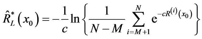
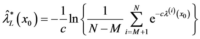
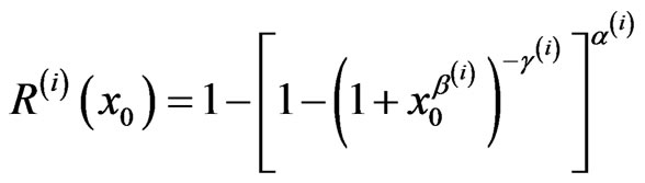
For a given time , the Bayes estimators of the SF and HRF are computed from
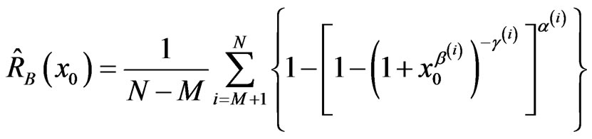 ,
,
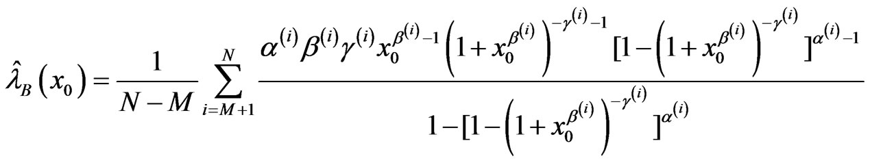 .
.
These are the Bayes estimators based on SEL function.
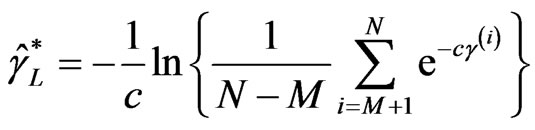
The Bayes estimators using MCMC method based on LINEX loss function are given by
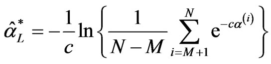 ,
,
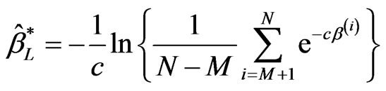 ,
,
 ,
,
 ,
,
 where
where
 ,
,
 .
.