Abstract

Here presented is constructive generalization of exponential Euler polynomial and exponential splines based on the interrelationship between the set of concepts of Eulerian polynomials, Eulerian numbers, and Eulerian fractions and the set of concepts related to spline functions. The applications of generalized exponential Euler polynomials in series transformations and expansions are also given.

1. Introduction

Eulerian polynomial is defined by the following equation (cf. for examples, [1-3]):

(1.1)

It is well-known that the Eulerian polynomial, , of degree can be written in the form

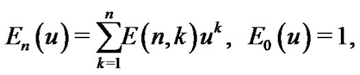(1.2)

where are called the Eulerian numbers that can be calculated by using

(1.3)

The Eulerian number gives the number of permutations of with permutation ascents (cf. [4]), or equivalently, the number of permutation runs of length (cf. [3]), where a set of ascending sequences in a permutation is called a run and is a permutation ascent if the th term in the permutation less than the st term. A geometric interpretation of Eulerian number were presented in [5] and [6], where which was found equaling to the volume of th slice of a -dimensional unit cubenamely,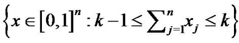. It is wellknown that the Eulerian fraction is a powerful tool in the study of the Eulerian numbers, Eulerian polynomial, Euler function and its generalization, Jordan function ( cf. [7]). The classical Eulerian fraction, , can be expressed in the form

(1.4)

spline functions are probably the most applicable one-dimensional polynomial spline functions. The values of spline functions can be defined as the volumes of slices of a -dimensional cube (cf. [8]). Hence, one can expect a tight connection between the Eulerian numbers and the spline function values. This is is one of the motivations to study the interrelationship between Eulerian polynomials and B-splines. Another motivation is from the construction of the exponential splines by using the exponential Euler polynomial discussed in [9], which will be described in this paper.

Polynomial spline functions can be considered as broken polynomials with certain smoothness, which are used to overcome the stiffness of polynomials, for instance the Runge phenomenon. One way to construct the univariate polynomial B-splines is using divided differences to truncated powers, and the truncated powers can be generated by iterated integrations. An extension called the truncated Tchebycheff functions can be constructed similarly using the iterated integrations with respect to positive, smooth weight functions, and the Tchebycheffian B-splines are linear combination of these truncated Tchebycheff functions. Exponential splines belong to a class of Tchebycheffian B-splines, which preserve many features of the polynomial B-splines such as smoothness, compact support, non-negativity, and local linear independence. One may find more details in [7,10,11] and [12] and some applications in [13] and [14]. In [15], Dyn and Ron considered periodic exponential B-splines defined by weight functions with, , and showed these B-splines possess a significant property of translation invariant and satisfy a generalized Hermite-Genocchi formula. Motivated by this work, Ron define the higher dimensional -directional exponential box splines in [16].

Another approach to construct the exponential splines to the base is using a linear combination of the translations of a polynomial B-spline with combination coefficients. The exponential splines to the base can be presented and evaluated by using exponential Euler polynomials, which connect to some famous generating functions (GF’s) in the combinatorics. The details can be found in Lecture 3 of [9-11], and Chapter 2 of [17], and we shall briefly quote them in next section. This approach can be used to derive a strong interrelationship between two different fields. For instance, in [18], the author presents the equivalence between exponential Euler polynomials, Euler-Frobenius polynomials, etc. and some frequently used concepts in combinatorics such as Eulerian fractions, Eulerian polynomials, etc., respectively, which will be surveyed as follows.

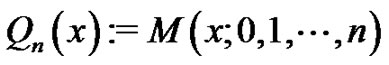
Let be an integer,. The symbol denotes the class of splines of order, i.e., functions satisfying the following conditions: 1) and 2) in each interval,where is the class of polynomials of degree not exceeding.

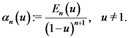
In the central part of Schoenberg’s lectures on “Cardinal Spline Interpolation” (CSI) (cf. [9]), the exponential Euler polynomial of degree to the base is defined as

(1.5)

where

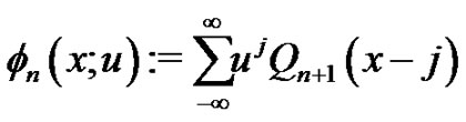
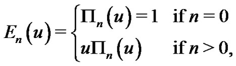
is the exponential spline of degree to the base, where

denote the cardinal forward B-splines. Here, an exponential spline means an element in satisfying the functional equation

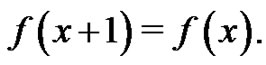(1.6)

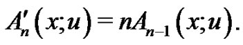
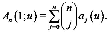
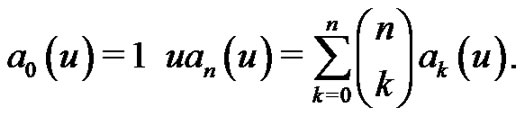
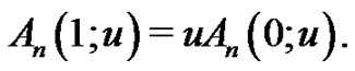
Obviously,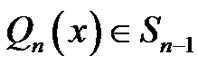. Therefore, , and it is easy to find satisfies (1.6).

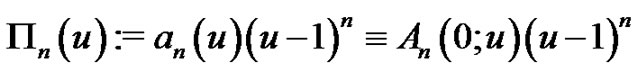
From [9], satisfies 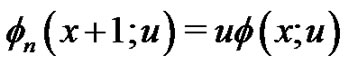and is a polynomial in the interval with the form

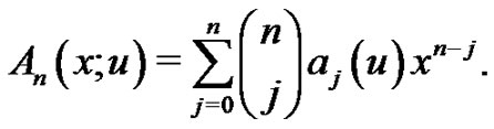
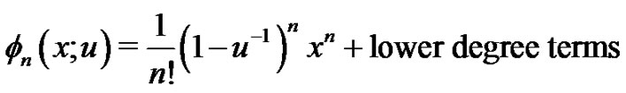
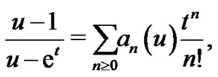
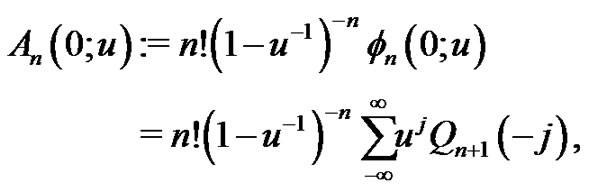
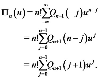
for. Hence, is a monic polynomial in. From [9], the generating function of is

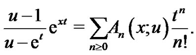(1.7)

Using (1.7) we may expand both sides of

and comparing the coefficients of power of in the expansions on two sides, we obtain

(1.8)

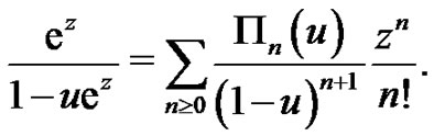
If, then (1.7) reduces to

(1.9)

where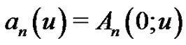. It is easy to see that

(1.10)

In particular,

(1.11)

Hence, we call the coefficient (polynomials) of the exponential Euler polynomial.

In addition, multiplying (1.9) by and comparing the coefficients of the powers of, we have the relations

(1.12)

Jointing (1.11) and (1.12) yields

(1.13)

If 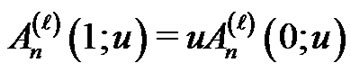for all integer, then (1.8) implies

.

Thus, we have

(1.14)

for all integer.

In the following, we call

(1.15)

the Euler-Frobenius polynomial. Since

(1.16)

defined by (1.15) can be written as

(1.17)

From (1.17), we know has zeros, all negative and simple, with a zero if and only if is. A proof can be found, for example, in [17].

On the other hand, from (1.9) and (1.15) we have

Transferring to, we change the above equation as

The left-hand side of the above equation can be expanded as

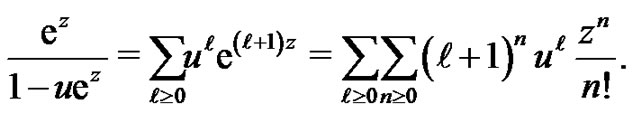
Comparing the right-hand sides of the last two equations yields

(1.18)

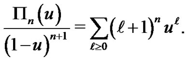(1.18) implies

(1.19)

In the introduction, we give the following definition of the Eulerian polynomial of degree, which is similar to (1.18).

(1.20)

where the Eulerian polynomial, 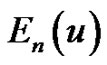can be written in the form of (1.2) with the Eulerian numbers calculated using (1.3).

In addition, Eulerian fraction, denoted by, is defined by

(1.21)

Comparing (1.18) and (1.20), (1.17) and (1.7), and (1.15) and (1.3), [18] gives the following results.

Proposition 1.1 [18] Let and be the polynomials defined by (1.15) and (1.9), respectively, and let Eulerian polynomials, Eulerian numbers, and Eulerian fractions be defined by (1.20), (1.2), and (1.21), respectively. Denote the cardinal forward B-spline of order by. Then we can set the relationship between the concepts as

(1.22)

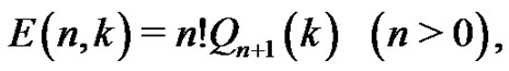(1.23)

(1.24)

As examples of the interrelationships shown in (1.22) - (1.24), we see

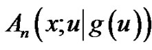
1)

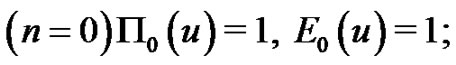
2)

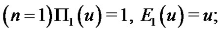
3) 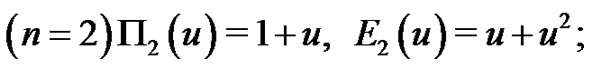etc.

and

1)

2)

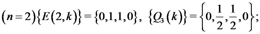
3)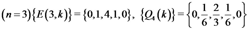; etc.

Using Proposition 1.1, [18] derives many properties of B-spline and Euler-Frobenius polynomials readily from the corresponding properties of Eulerian polynomials and Eulerian numbers, and vice versa. Applications in B-spline interpolation and evaluation of Riemann Zeta function values at odd integers are also given in [18].

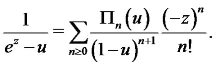
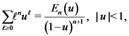
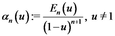
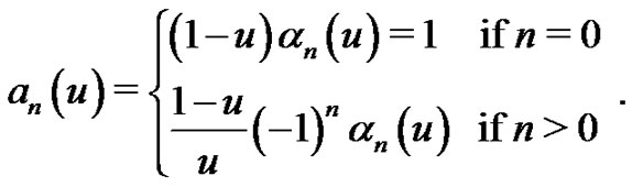
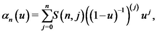
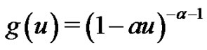
Let. It is well-known that the Eulerian fraction defined by (1.21) can be written as

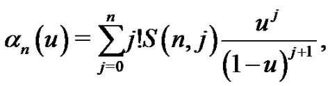(1.25)

where are the Stirling numbers of the second kind, i.e., 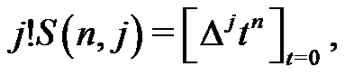or equivalently, the number of partitions of distinct elements in blocks.

The connection shown in Proposition 1.1 also provides some important applications, shown in Section 2, of B-splines and exponential B-splines to the enumerative combinatorics. In the section, a generalized Eulerian fraction and a generalized exponential spline to the base are derived. Section 3 discusses the applications of the generalized exponential Euler polynomials in the series transformations and expansions. Furthermore, using the combinatorial technique, we may generate exponential splines in higher dimensional setting, which will be briefly described at the end of the section and will be discussed in a later paper on the multivariate spline functions.

2. Generalized Exponential Splines

In this section, we will introduce a generalized Eulerian fraction, from which a generalized exponential spline to the base will be derived. We shall also discuss the corresponding generalized Euler-Frobenius polynomials and their applications.

It is obvious that (1.25) is equivalently

(2.1)

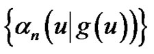
where. Hence, we may extend the Eulerian fraction to a more general case, which will be denoted by and called generalized Eulerian fractions associated with an infinitely differentiable function:

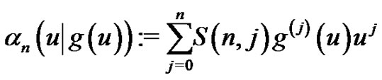(2.2)

Therefore,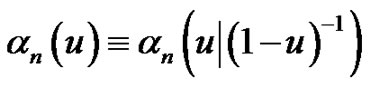. An analogue of the coefficients of the exponential Euler polynomials defined by (1.10) is extended to

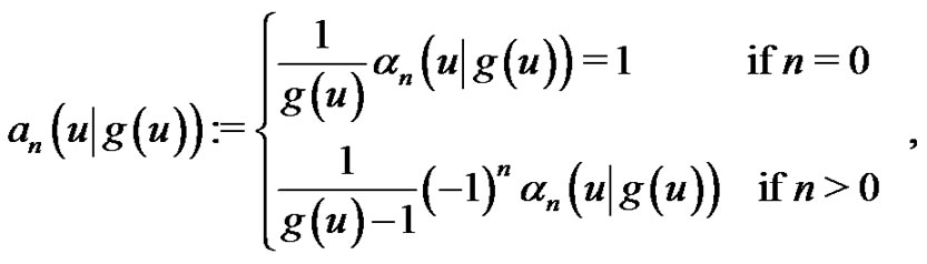(2.3)

which is associated with an analytic function.

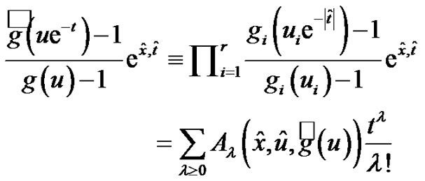
We now find the generating function of

and.

Theorem 2.1 Let be an infinitely differentiable function, and let and be defined by (2.2) and (2.3), respectively. Then their exponential generating functions are

(2.4)

and

(2.5)

where.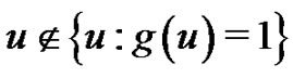

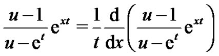
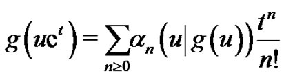
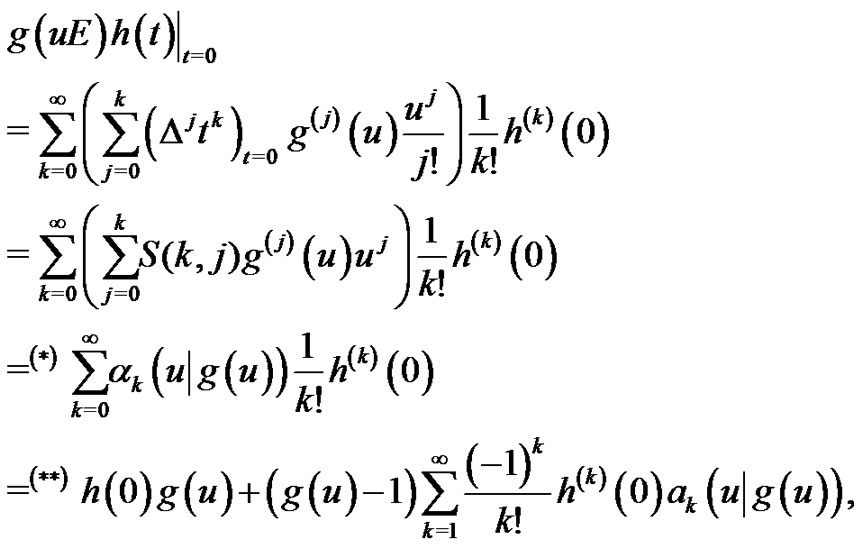
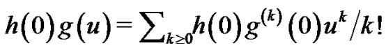
Proof. Substituting (2.2) into the right-hand side of (2.4) and using the generalized Euler series transform formula (cf. [19] and (3.1) in [20]), we can evaluate the exponential generating function of formally as

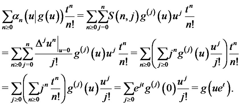
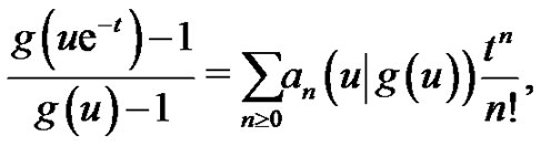
Similarly, by substituting (2.3) into the right-hand side of (2.5) and applying formula (2.4) to the resulting expression, we have

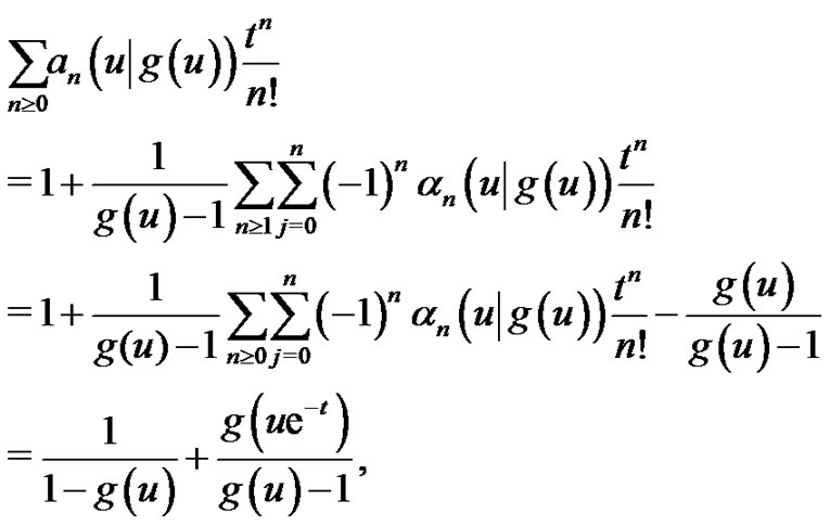
which yields (2.5) and completes the proof of the theorem.

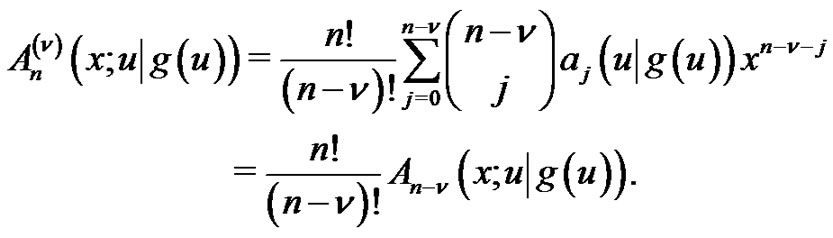
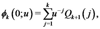
From we now construct polynomials

for using the following expansion.

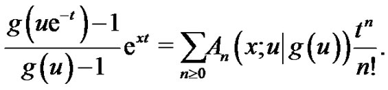(2.6)

Thus, can be evaluated from 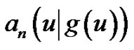as follows.

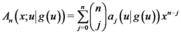(2.7)

for. In particular, 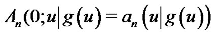and

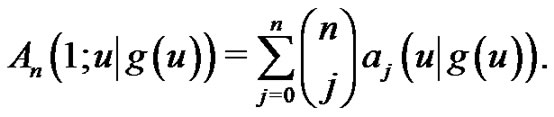
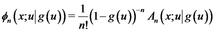
We call the generalized exponential Euler polynomial of degree associated with to the base, and the coefficient of

. In addition, we call the generalized Euler polynomials, and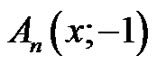, the regular Euler polynomials, are the special case of 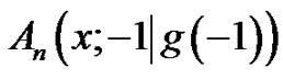for.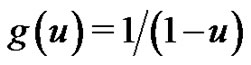

A generalized exponential spline function to the base, denoted by, is therefore defined using () as follows.

(2.8)

in. However, if one wants to extend to all real associated with such that, needs to satisfy some periodic conditions. Let us consider the class of

with real constants and.

Then we have the following result.

Theorem 2.2 Let function be defined by (2.8) on associated withwhere and are real constants and, can be extended to a continuous function for all real if and only if. Furthermore, the extension is fulfilled by the functional equation

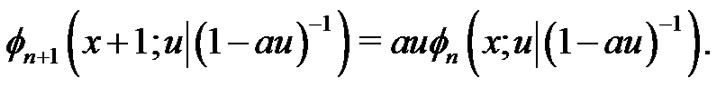(2.9)

Proof. From [9], for (2.9) combined with the condition that require

to satisfy in the periodic conditions

(2.10)

for. From (2.7), we have

Hence, condition (2.10) is equivalent to

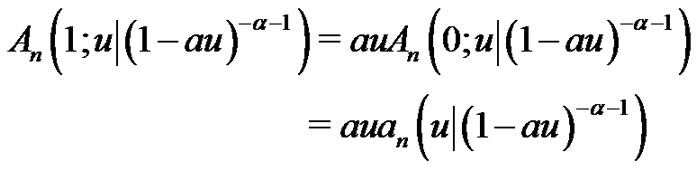(2.11)

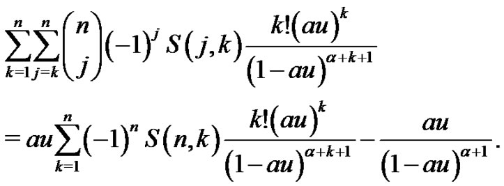
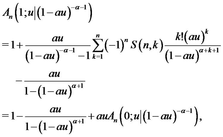
for all. From (2.7) (2.3), and (2.2), we have

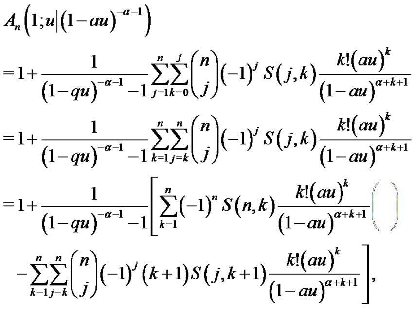(2.12)

where the last step is due to the identities

and

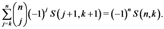
The double sum in the rightmost expression of (2.12) can be further changed to

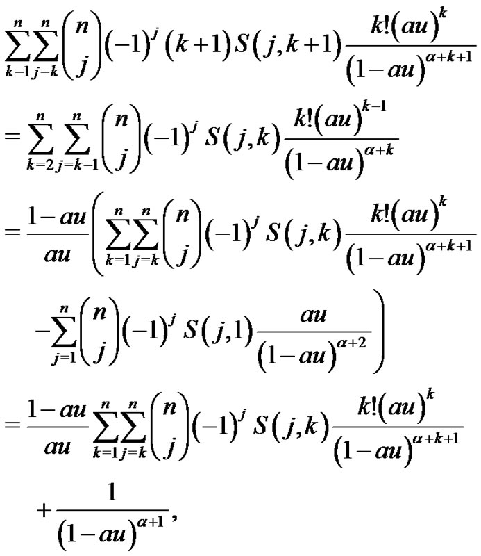
where the last step comes from 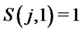for all. Substituting the last expression of the double sum

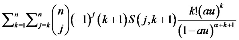into equation

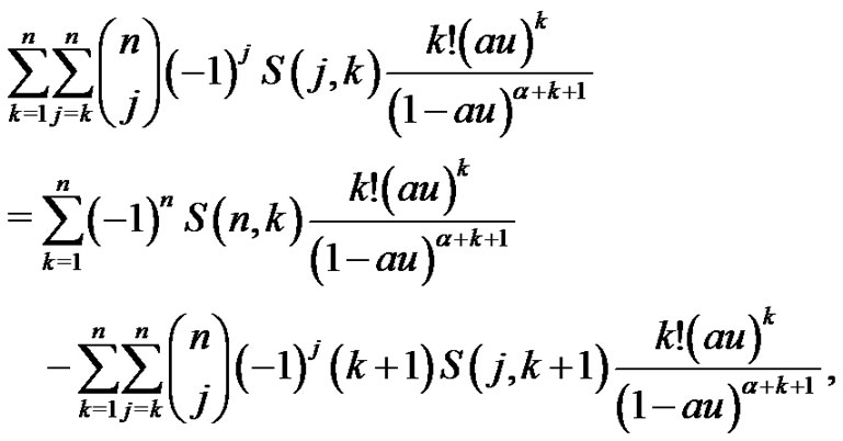
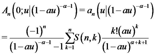
which comes from (2.12), and solving the resulting equation for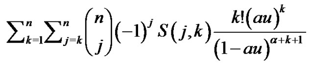, we obtain

(2.13)

Substituting the last equation to the first equation of (2.12) yields

where the last step is implied by

(see (2.2) and (2.3). Therefore, if

, then

. The sufficiency is obvious. This completes the proof of the theorem.

Remark 3.1 Other generalized exponential splines are planed to be constructed. And the properties of the exponential splines need to be investigated.

3. Applications in Series Transformations and Expansions

All formulas presented in this section are formal identities in which we always assume that or according as or appears in the formulas.

Theorem 3.1 Let and be infinitely differentiable on, and let () be the generalized exponential Euler polynomial to the base defined by (2.6) or (2.7). Then we have formally

(3.1)

where is not any poles of and for any.

Proof. First, we apply the operator to the infinitely differentiable function at, where is the shift operator.

On the other hand, we can present

By applying (3.1) in [19] to the inner sum of the rightmost side of the above equation for and noting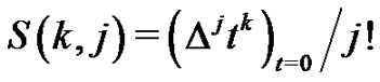, we obtain

which implies (3.1) by writing

formally, where for and we use (2.2) and (2.3), respectively. This completes the proof of the theorem.

Remark 4.1 The series transformation formulas (3.1) have numerous applications by setting different infinitely differentiable functions for. For instance, If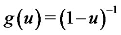, then (3.1) becomes to

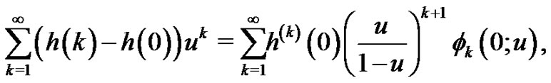(3.2)

where and the relation (1.5) has been used.

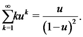
Evidently, when is a polynomial, formulas (3.1) and (3.2) become closed form of summation formulas with a finite number of terms. Moreover, the Right-hand side of each formula may also be viewed as a for the sequence of coefficeients contained in the power series on the left-hand side. For example, if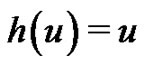, noting

we have

At the end of this section, we will show a way to extend our construction of exponential splines to the higher dimensional setting. First, we shall adopt the multi-index notational system. Denote

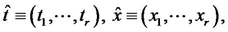
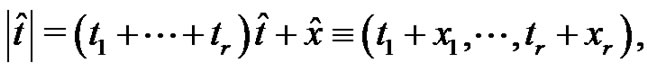
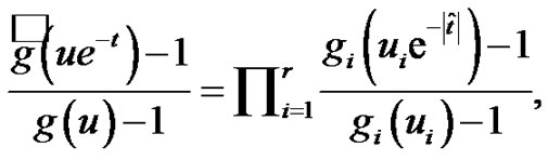
Moreover, we write with being non-negative integers. Also, means , and means for all.

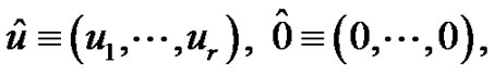
We now define a generalized higher dimensional exponential polynomials as follows.

Definition 3.2 Let 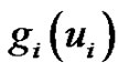be any given formal power series over the complex number field with.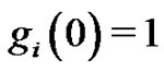

Then 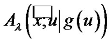defined by

(3.3)

are called the generalized higher dimensional exponential Euler polynomials of degree associated with to the base, where. In particular, for, (3.3) defines higher dimensional exponential Euler polynomials of degree to the base by

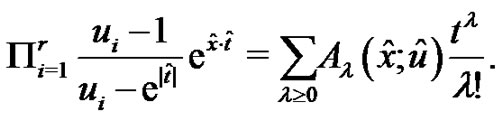(3.4)

Let. Then the polynomial defined by (3.4) is called the higher dimensional (regular) Euler polynomial of degree. The more details will be given in a later paper.

4. Acknowledgments

The author greatly appreciate the discussion with Carl deBoor since 2005 and the valuable suggestions and the lecture [17] he offered fervently.

5. References

[1] L. Carlitz, D. P. Roselle and R. Scoville, “Permutations and Sequences with Repetitions by Number of Increase,” Journal of Combinatorial Theory, Vol. 1, No. 3, 1966, pp. 350-374. doi:10.1016/S0021-9800(66)80057-1

[2] L. Carlitz, “Eulerian Numbers and Polynomials of Higher Order,” Duke Mathematical Journal, Vol. 27, 1960, pp. 401-423.

[3] L. Comtet, “Advanced Combinatorics: The Art of Finite and Infinite expansions,” Springer, Dordrecht, 1974.

[4] R. L. Graham, D. E. Knuth and O. Patashnik, “Concrete Mathematics,” A Foundation for Computer Science, 2nd Edition, Addison-Wesley, 1994, pp. 267-272.

[5] D. Foata, “Distribution Eulérienne et Mahoniennes sur le Groups des Permutations,” Proceedings of the NATO Advanced Study Institute, Berlin, 1-10 September 1976, pp. 27-49.

[6] R. P. Stanley, “Eulerian Partitions of a Unit Hypercube,” Proceedings of the NATO Advanced Study Institute, Boston, 1977, p. 49.

[7] G. Birkhoff and C. de Boor, “Piecewise Polynomial Interpolation and Approximation,” Approximation of Functions, Elsevier Publishing Company, Amsterdam, 1964, pp. 164-190.

[8] C. de Boor, K. Hllig, S. Riemenschneider, “Box Splines. Applied Mathematical Sciences,” Springer-Verlag, New York, 1993.

[9] I. J. Schoenberg, “Cardinal Spline Interpolation,” CBMSNSF Regional Conference Series in Applied Mathematics, 1973.

[10] C. de Boor, “On the Cardinal Spline Interpolant to e^iut,” SIAM Journal on Mathematics Analysis, Vol. 7, no. 6, 1976, pp. 930-941. doi:10.1137/0507073

[11] C. de Boor, “A Practical Guide to Splines,” Revised Edition. Applied Mathematical Sciences, Springer-Verlag, Hoboken, 2001.

[12] L. Schumaker, “Spline Functions: Basic Theory,” John Wiley & Sons, New York, 1981.

[13] O. A. Vasicek and H. G. Fong, “Term Structure Modeling Using Exponential Splines,” The Journal of Finance, Vol. 37, No. 2, pp. 339-348. doi:10.2307/2327333

[14] C. Zoppou, S. Roberts and R. J. Renka, “Exponential Spline Interpolation in Characteristic Based Scheme for Solving the Advective-Diffusion Equation,” International Journal of Numerical Methods in Fluids, Vol. 33, No. 3, 2000, pp. 429-452. doi:10.1002/1097-0363(20000615)33:3<429::AID-FLD60>3.0.CO;2-1

[15] N. Dyn and A. Ron, “Recurrence Relations for Tchebycheffian B-splines,” Journal d'Analyse Mathématique, Vol. 51, 1988, pp. 118-138. doi:10.1007/BF02791121

[16] A. Ron, “Exponential Box Splines,” Constructive Approximation, Vol. 4, no. 4, 1988, pp. 357-378. doi:10.1007/BF02075467

[17] C. de Boor, “Chapter II. Splines with Uniform Knots,” draft jul74, TeXed, 1997.

[18] T. X. He, “Eulerian Polynomials and B-splines,” ICCAM-2010, University of Leuven, Belgium, 5-9 July 2010.

[19] T. X. He, L. C. Hsu, P. J.-S. Shiue and D. C. Torney, “A Symbolic Operator Approach to Several Summation Formulas for Power Series,” Journal of Computational and Applied Mathematics, Vol. 177, 2005, pp. 17-33. doi:10.1016/j.cam.2004.08.002

[20] T. X. He, L. C. Hsu and P. J.-S. Shiue, “A Symbolic Operator Approach to Several Summation Formulas for Power Series II,” Discrete Mathematics, Vol. 308, No.16, 2008, pp. 3427-3440. doi:10.1016/j.disc.2007.07.001