Optics and Photonics Journal
Vol.06 No.10(2016), Article ID:71210,24 pages
10.4236/opj.2016.610025
Static Laser Light Scattering Studies from Red Blood Cells
David Joseph, Amit Kumar
Optical Engineering Section, Department of Applied Physics, Guru Jambheshwar University of Science and Technology, Haryana, India

Copyright © 2016 by authors and Scientific Research Publishing Inc.
This work is licensed under the Creative Commons Attribution International License (CC BY 4.0).
http://creativecommons.org/licenses/by/4.0/


Received: June 23, 2016; Accepted: October 11, 2016; Published: October 14, 2016
ABSTRACT
A homemade Static Light scattering studies has been used to determine angle resolved scattered intensity for different polarization states of the incident laser light. Classical light scattering set ups are being used to study morphological aspects of scatterers using simple set ups using low power lasers. Red blood cells form rather interesting as well as a challenging system for scattering experiments. The scattering spectrometer consists of a scattering arm, a scattering turn table and collimating arm. Along with polarizers integrated in the collimating arm as well as scattering arms ensures collection of scattered flux with the required polarization state. This technique is being developed for its in vitro studies using fresh red blood cells. A brief review of the theoretical models used for scattering from Red Blood Cells (RBC) has been discussed in the paper. Scattering pattern (scattering plots) as well as polar plots of scattered flux have been determined for different polarization state of the incident light. Insight into the orientation of major axis of particles can be inferred from the polar plots.
Keywords:
Raleigh Scattering, Mie Scattering Red Blood Cells, Polar Plots, Clustering, Circularly Polarized Light, Linearly Polarized Light, Polarizer, Scattering Turn Table, Collimator Arm, Scattering Arm

1. Introduction
Static light scattering is a classical field the birth of which may be assigned to Rayleigh scattering and the explanation of blueness of sky [1] [2] . This novel formulation made demarcation as an elastic scattering event and inelastic scattering event. Keeping in mind the non destructive scattering, one would find immense applications and their techniques that are biologically important processes. Along with X-ray scattering, light scattering has emerged as a potent tool for probing soft matter materials. Depending on the size of particles, Raleigh Gans, or Mie scattering regimes can be defined [3] - [6] . The size, orientation and the refractive indices decide the scattering event and corresponding scattering matrix elements are defined as below.
The scattering in any direction is described by four amplitude functions, S1, S2, S3 and S4 all functions of θ and f which form a matrix S(θ, f) of four elements. The definition of S(θ, f) is
 (1)
(1)
The corresponding intensity matrix F has 16 elements. By making θ = 0, we obtain the four complex matrix components S2(0), S2(0), S3(0), S4(0) forming the matrix S(0) of four elements. The electric field at a point P beyond the slab is
 (2)
(2)
where q = 2pNlk−2.
In red blood cells, the size typically varies from 6 μ to 8 μ and has a biconcave disc shape. An ensemble of randomly oriented dilute Red Blood Cells (RBC) will therefore be well suited model system for scattering.
The spatial arrangement of particles comes to picture, when one takes into account the scattering from multiple particles. While single particle scattering takes into account the scattering from simple particles, multiple scattering has been always a mathematical difficulty. Experimentally, for multiple scattering events, it is difficult to convolute for different scattering events. With a perspective of colloidal interactions, it is well characterized by the pair potential existing between the particles which is well known from DLVO theory for colloids. Even though the nature of potential is not well known, the Derjaguin, Landau, Verwey and Overbook (DLVO) potential along with the Resealed Mean spherical approximation by Henson and Hayter provides a good model to explain the many particle interaction and stability of particle in a medium [7] [8] .
In the opposite regime, if the attractive forces dominate, the particles tent to become clusters. These clusters in the case of red blood cell (RBC) clusters arc called rouleaux [9] . The work in the area of scattering from cells has been carried established by Valery Tuchin and his group [10] [11] . Theoretical and experimental work of Preizchev et al. on Red Blood Cells (RBC) throws light into the morphological features of RBC [12] . Britton chance and Alfano has extended the scattering technique to high potential biological applications [13] [14] . Alfano et al. have elaborately studied the florescence in tissues along with its scattering effects while propagating in a biological medium. William Bickel has elaborately focused his studies on the shape and size of the particle using the scattering matrix method taking almost all shapes into consideration [15] . George Benedick has also shown immense applications of SLS studying macromolecules [16] . The morphological changes of the RBC cells with the malarial parasite infection has been studied by the Felt group at MIT, USA [17] . On the contrary, clustering of particles to form fractal can be studied by a formulation due to Sorensen et al. where they have determined the clusters grown by diffusion limited aggregation (DLA) [18] . Depending upon the clustering dynamics, clustering process can be Diffusion limited Aggregation (DLA) or Reaction Limited Aggregation (RLA) [19] - [21] and correspondingly, the fractal dimensions will be different. The focus of the present work is however limited to single particle scattering and determination of its form factor. The Red Blood cells RBC are heavily prone to physical and pathological conditions in the blood plasma such as ionic variations, pH variations, temperature variations and pathological conditions. Consequently, the RBC can change its shape and size, or can form clusters (see Figure 1).
The normal disc shaped red blood cells are shown in Figure 2.
Another situation is the sickle cell anemia in which the RBC takes the shape of sickle (see Figure 3). Further RBC of animals, birds, reptiles all will be interesting in its own.
2. Scattered Light―In General
A typical set-up for the static light scattering experiment consist of a laser beam illuminating a sample and a detector set up at scattering angle θ measuring the intensity

Figure 1. (a) Normal surface view (b) Rouleaux formation (c) rendering spherical by water (d) crenate structure by the influence of NaCI (d) abnormal structure which do not occur in body normally.
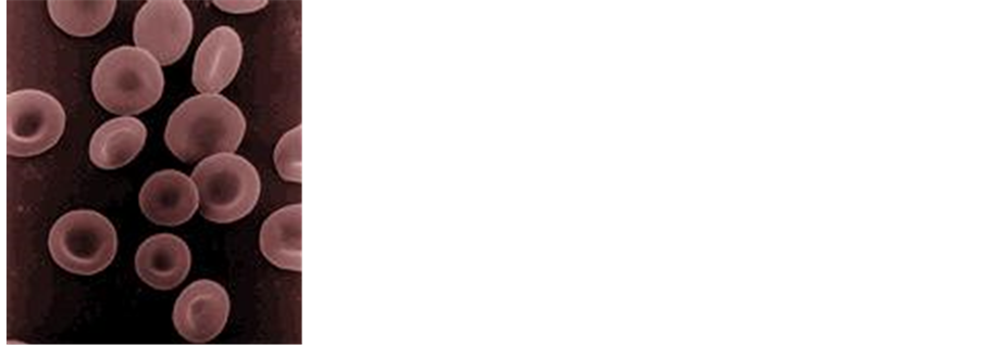
Figure 2. Normal Red blood cell with disc shape.
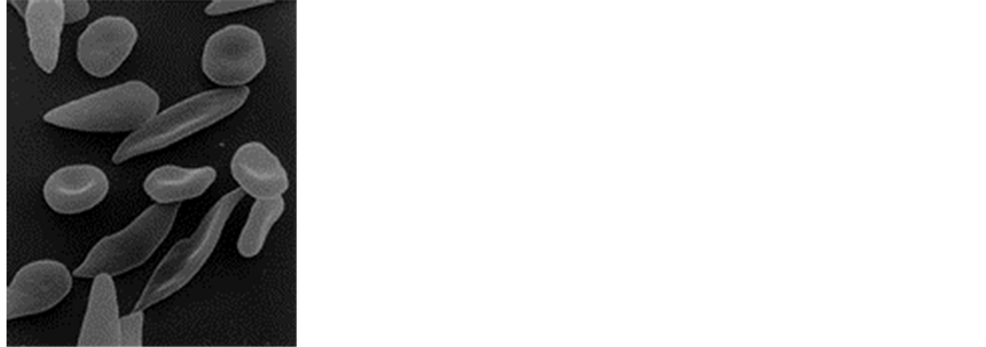
Figure 3. Red blood cells disc shaped (normal cells) along with sickle cell Anemia blood cells.
I(θ, t) of the scattered light [22] . Typically, the incident and scattered beams are shaped by apertures, slits, or by optics such as lenses. Usually, the incident beam is vertically polarized as the detector moves in a horizontal plane defining the scattering plane. The intersection region of the sample which is illuminated by both incident and scattered beam is defined as the “scattering volume”. Figure 4 shows a scheme of a classical light-scattering set-up, where the incident light is a plane electromagnetic wave,
 (3)
(3)
Here Ei(r, t) is the electric field, E0 is the Amplitude and I denotes the incident light intensity. The polarization ni is perpendicular to scattering plane. ki is the incident light wave vector ki = 2πn/λi and ωi is the angular frequency which varies in time.
In a colloidal state, if the particles are charged to form ordering, and if we ignore multiple scattering, the scattered electric field may be written simply as a summation:
 (4)
(4)
Here is ωi written as ω because the scattering is elastic.
Light scattering from blood or of tissues are important in many medical applications. The light diffusion in tissues or cell suspension is important photodymanic laser therapy [1] - [3] . Recently, light scattering spectroscopy (static light scattering or Dymanic light scattering) has attracted much interest [4] - [6] . In situ analysis of RBC is useful tools for diagnostics of many blood related diseases. Among these analysis, optical measurement on blood, both in vivo and in vitro, is a growing field, since useful information can be extracted with rather simple and nondestructive measurement procedures. A good understanding of the interaction of light with blood is a prerequisite for optical blood analysis. Blood optics is special in several ways, motivating special efforts in improving the understanding of light transportation in blood. Light is heavily scattered by non-spherical red blood cells (RBCs), not containing any scattering internal structures. Aggregation of RBCs are also known to alter light propagation through blood; however the structural aspects of the aggregates or clusters are not well studied.
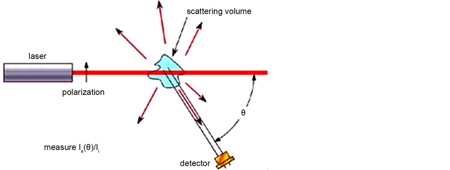
Figure 4. Typical light scattering experiment.
It is known that the scattering and absorption of light in blood are largely governed by the red blood cells. It is the refractive index of RBCs, as well as their size, shape and orientation that determine how light propagates. The size of an RBC is typically 6 - 10 wavelengths in the optical region and the full wave methods require fast computers with large RAM, when applied to such large objects. The contrast between the blood cell and the surrounding plasma is quite small. For scattering at a vacuum wavelength of 630 nm the typical values for the index of refraction is 1.40 for a blood cell and 1.35 for the plasma. Thus the blood cell forms a weakly scattering system. The different methods used to model RBC are described as follows:
1) FDTD method
2) The T-matrix method
3) Mie scattering
4) DDA method
5) The superposition approximation,
6) The Rytov approximation.
In general, the normal RBC shape is modeled as discocyte, i.e. an axially symmetric disk, slightly indented on the axis and having the mirror plane symmetry perpendicular to the axis. The information from these calculations is useful in the development of models of light propagation in whole blood containing many RBC.
3. Preliminaries of Simulation Methods
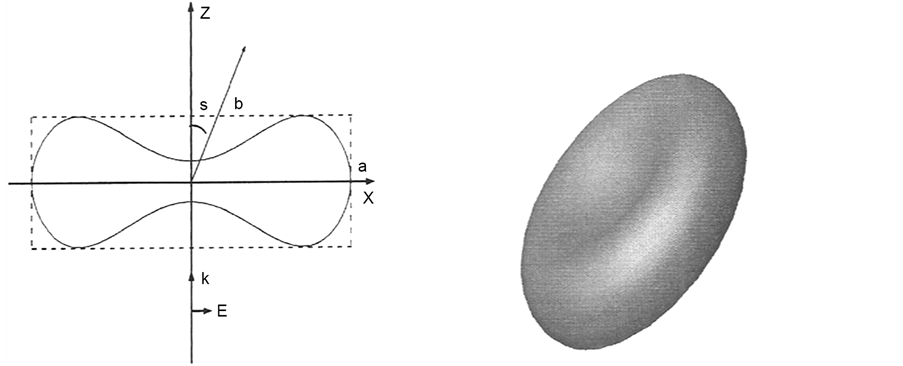
In the simulations the refractive index for the RBC is set to n1 = 1.406 and the refractive index of the surrounding blood plasma is set to n2 = 1.345. The absorption is neglected in both regions. The model of the disk-like normal RBC used in the simulations is defined in the references [13] [14] with a volume of the RBC as 94 mm3. The membrane of RBC has a negligible influence on the scattered field, and hence the RBC models do not include the membrane or any other internal structure. Figure 5 shows the cross section of the disk-like RBC model, where the enclosing box has height a = 2.547 mm and length b = 7.76 mm. The three-dimensional (3D) shape is obtained by rotating the
 (a) (b)
Figure 5. (a) showing the rotator cases of RBC; (b) 3D picture of RBC.
cross section around the z axis. Figure 5(b) depicts the 3D picture of the disk-like RBC model. In the simulations, the incident wave is a time-harmonic linearly polarized plane wave. It propagates in the positive z-direction with the electric field in the x-direction. The complex incident electric field is given by
 (5)
(5)
where k = n2w/c0 is the wave number for the plasma and c0 is the velocity of light in vacuum. The RBC is rotated around the y―direction in order to change the angle of incidence. The rotation angle of the axis of symmetry relative to the z-direction is denoted θi.
The scattering probability was calculated as a function of the zenith scattering angle θs This scattering probability, P(θs), was calculated by numerical integration of the differential scattering cross section, σdiff(θs, fs), over all azimuthal angles fξ[0, 2π]:
 . (6)
. (6)
The differential cross section is defined as the time averages of the Poynting vector of the scattered and incident fields, respectively. Furthermore, r is the radial unit vector, E(r, θ, f) is the scattered electric field, H*(r, θ, f) is the complex conjugate of the

where
 (7)
(7)
Corresponding magnetic field. and n0 = 120 πΩ is the wave impedance of vacuum.
3.1. FDTD: Yee’s Method
The FDTD algorithm was originally proposed by K. S. Yee in 1966 [17] . Detail of FDTD can be found in the book written by Taflove [22] , Which gives a good overview. The FDTD algorithm numerically solves the Maxwell’s curl equations in time domain. In the 3D case, the Maxwell’s curl equations are discretized in time and space, resulting in six coupled scalar finite-difference equations in Cartesian coordinates. All three electric field components and all three magnetic components are spatially allocated (Figure 6). The electric and magnetic fields are temporally offset and stepped in a leap frog scheme using the finite-difference form of the curl operator. In order to get the angular far-field distribution of the scattered light, several techniques are required:
3.1.1. Absorbing Boundary Condition (ABC)
Because of the finite computational domain, the values of the fields on the boundaries must be defined so that the solution region appears to extend infinitely in all directions. With no truncation conditions, the scattered waves will be artificially reflected at the boundaries leading to inaccurate results. The perfectly matched layer (PML) ABC suggested by Berenger [23] have been implemented in the three-dimensional FDTD program and is used in the examples in the paper.
3.1.2. Total Field/Scattered Field
The field formulation forms the basis of this formulation which considers the scattering patterns and computes the corresponding total field/scattered fields. The computational grid are created for computations and is divided into two regions. The total field region encloses the scattering particles. whereas in the scattered field region, only the scattered field matrix are stored. At the boundary between the two regions, special boundary conditions are needed to connect the fields in different regions. Here, the incident field is either added or subtracted from the total field. The conditions used for the simulations in the paper are described in detail in Ref [22] . The schematic of the fields are given in Figure 7.
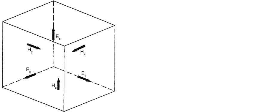
Figure 6. Total field/scattered field regions.
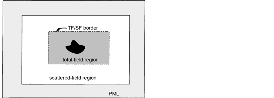
Figure 7. Schematic of total field/Scattered field description.
3.1.3. Far-Field Transformation
The FDTD is inherently a near-field method. To determine the far-field scattering pattern, the near-field data is transformed to the far-field by the near-field to far-field (NFFF) transformation. The details of the NFFF technique can be found in [22] .
3.2. The T-Matrix Method
This method as known as null field method was formulated by Waterman [23] . This method computes the surface fields on a spherical unit surface. The incident, reflected, and internal fields are expanded in terms of vector wave functions. Boundary conditions are used to derive a relation between the expansion coefficients of the scattered and of the incident fields. The coefficients of the fields are related by a matrix referred to as the T-matrix. The method is very efficient for objects that have size that are less than a few wavelengths in diameter. The calculations converges for larger objects also, but then the size of the matrix increases. T-matrix method is applied to the scattering from blood cells in the shape of oblate spheroids in ref: [24] . A computer code developed by Barber et al. [25] was used for these calculations with Quadruple precisions using real numbers with 32 digits precision. However, getting accurate results for blood cells with realistic shape is not easy by this method. Nevertheless, this method works faster than e.g., FDTD method.
3.3. Mie Scattering
Mie scattering is celebrated a theory formulated by Gustav Mie [6] , developed initially for spherical scatterers. The formulation is based incident field and the unknown internal field that are expanded as regular vector waves. The unknown scattered field is expanded as outgoing vector waves. The relation between the expansion coefficients for the incident and scattered fields are derived considering the boundary conditions applicable at the spherical surface. The relation is then given by a diagonal matrix and the T-matrix for the sphere is derived. T-matrix is diagonal and so one does not get the same numerical problems that occur for non-spherical objects. Numerical results can also be obtained for very large spheres, and the calculations are very fast. Mie scattering is often considered as exact calculations and is used as a reference method to compare with other numerical methods.
3.4. The Discrete Dipole Approximation
The Discrete Dipole Approximation (DDA) is closely related to the method of moments. The original derivation of the method is less rigorous and does not rely on the volume integral equation. The principle of the method is as follows: The scattering volume is divided into N parts, each part is small enough to be represented by a dipole moment. The induced dipole moment of each volume element is equal to the electric field in the volume multiplied by the polarizability of the volume. The electric field is a superposition of the fields from the sources external to the object and the electric fields from the sources inside the object. The field from the external sources is the incident plane wave and hence the electric field in a volume j is given by
 (8)
(8)
where in the term  is the Electric field at a position rj from a dipole P(rk). It can be found in basic textbooks in electromagnetic theory. In iteration method i.e. the conjugate gradient method is applied to solve the equations. More details can be found in the references [26] [27] .
3.5. Superposition Approximation
The superposition approximation is based on the assumption that multiple scattering effects are small within the cell. The scattering object may be divided into several parts each part being a scattering objects. The multiple scattering effects between the objects are neglected. The advantage is that the volume of the scattering objects is reduced implying a reduction of the CPU-time and the required RAM of the computer. In the example a blood cell was divided in two halves through the yz-plane. The far-field pattern Ef in yz-plane for each half was calculated by the FDTD method. Then the two far-fields were added and compared with the same far-field from the whole blood cell. The patterns agree very well. The far fields are the same except for the phase shifts. The superposition approximation facilitates the calculation of far-fields for one RBC and then sum up for phase shifts to get the far fields for the RBCs. The far field approximation is thus calculated using the equation:
 (9)
(9)
where r is the translational vector of RBC n relative to the origin.
3.6. The Rytop Approximation
The Rytop approximation is a frequently used method in tomography [28] [29] . It is used for inverse scattering problem. This method can be explained as follow. Consider an object occupies a volume V, and let refractive index be n1 for the object and n2 for the surrounding medium. The approximation assumes that when the wave passes the object, the phases of two waves are shifted while its amplitude and polarization are unaltered. The wave is assumed to travel as straight rays parallel to z-axis, Let d(x, y) be the total distance that ray travel inside scattering object. If z = z1 is a plane behind the object, the total electric field in that plane may be computed as
 (10)
(10)
Thus the phase is shifted to an angle  compared to an incident wave. The far field amplitude is given by the near field to far field transformation as.
 (11)
(11)
where S is the plane z = z1. All reflection of the wave is neglected. The approximation gives far field amplitude that is only accurate for the angles θs < π/2. The code for the far field amplitude is very simple and short and for that reason this method is alternative to far more time and memory requiring full wave methods.
4. Experimental
It consists of homemade light scattering Spectrometer in which a laboratory available spectrometer has been modified for acting as the scattering setup. The set up is a classical light scattering setup with a 1) Collimating Arm, 2) Scattering Turn Table, 3) Scattering Arm.
This has been shown in Figure 8 and will be discussed below.
4.1. Collimating Arm
Collimating Arm consists of a pinhole tube sufficiently wide for the laser beam to pass through and is made up of a aluminum. Following this is a lens and a polarizer system. The polarizer can be rotated in the collimating arm, so as to get required polarization state for the incident laser beam. A separate circular polarizer (quarter wave plate) can be inserted whenever one needs circular polarized light. By setting the polarizer and the circular polarizer one can get circular or a elliptical polarized light.
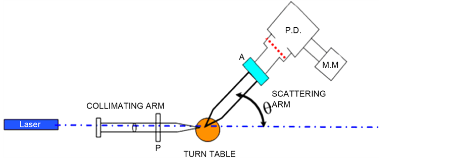
Figure 8. Experimental setup. P is polarizer, A = Analyzer, PD = Photo Diode, M.M. is the Multimeter.
4.2. Scattering Turn Table
Scattering Turn Table consist of the angular turn table of Spectrometer and the scattering cell holder. A cell holder has been fabricated so that light can enter the cell and scattering data can be obtained at different angles around the cell.
4.3. Scattering Arm
Scattering Arm consists of a pin hole which collects the scattered flux from the scattering cell. The scattered light flux is collected in the same plane as the incident light flux. The scattered light is collected by the lens and iris diaphragm, and further the scattered light is fed to a photo diode. The iris can be opened or closed, as on our will. In between the lens and the iris, a polarizer is again introduced so as to get vertical-vertical (VV) for horizontal-horizontal (HH) or vertical-horizontal (VH) polarization state. The laser used here is a 2 mV Helium Neon laser with 632.5 nm wavelength. The full photograph of experimental setup is shown in Figure 8.
4.4. Sample Preparation
Sample preparation has been done in the university health centre. Human blood (5 ml) was injected out into a centrifuging tube and was citrated with sodium citrate solution. This was rotated at 3000 rpm. Blood plasma from this has been removed, and 1 ml of Red Blood Cell (RBC) has been injected out to a separate tube. This has been diluted (as required) to make a very dilute system. It has been insured that the RBC cells do not aggregate. This is done by using a buffer as the diluting liquid. The pH has been kept at a value around 7.0. Glass cell of about 8 mm outer diameter has been fabricated for this work. The scattering data is typically collected between angles (θ) of 20˚ to 130˚ with an increment of 5˚. Since the cells remain alive approximately for 3 hours, the experiments are to be finished before three hours. The photograph of the set up is shown in Figure 9.
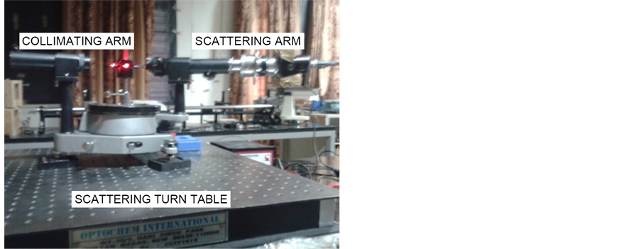
Figure 9. The fabricated Experimental Static Light Scattering setup. Collimating arm (with the polarizer), Scattering arm (with analyzer, Iris diaphragm, and Detector). The cell can be seen in the middle.
Angle resolved scattered Intensity have been determined and plots have been plotted between Scattered Intensity Vs Angle for
1) Unpolarized Incident light
2) Vertically Incident polarized light
3) Circularly Incident polarized light
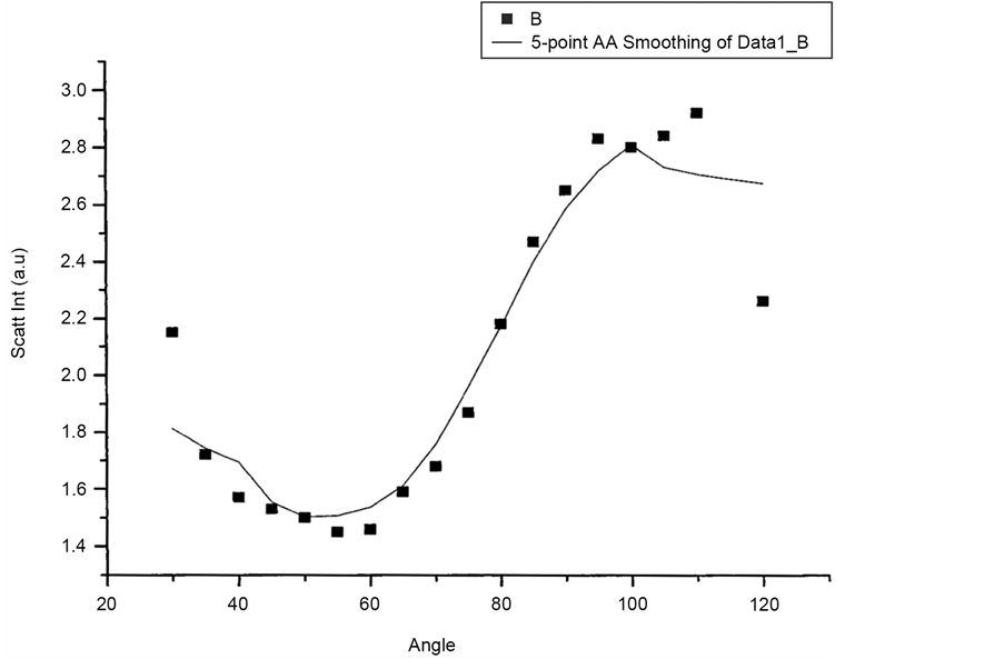
Figure 10 and Figure 11 show Scattered Intensity Vs Angle plots for unpolarized incident light with the scattering arm collecting horizontally polarized light and vertically polarized light respectively. The scattered intensity variations in the two plots are similar.
Figure 12 and Figure 13 shows scattered flux variation with angle for vertically polarized Incident light, collecting Horizontal and Vertical polarized light respectively as VH and VV component. These two graphs (Figure 12 and Figure 13) also show similar variation. Figure 14(a) and Figure 14(b) scattered intensity variation with angle for circularly polarized Incident light collecting scattered intensity for horizontally polarized (CH) and vertically polarized (CV). These two plots Figure 14(a) and Figure 14(b) also showing similar variation.
4.5. Polar Plots
4.5.1. Case 1: Unpolarized Incident Light
Polar plots are plotted by first fixing an angle (θ = 30˚, 60˚, 90˚, 120˚) and then varying the Azimuthal angle (φ) by rotating the Analyzer in the scattering arm. Figure 15 and Figure 16 shows the polar plot for the angle (θ = 30˚, 60˚) for incident Unpolarized light. The scattered intensity for azimuthal angle (φ = 50˚) shows higher scattering value for scattered flux in these two polar plots for unploarized light.
4.5.2. Case 2: Circularly Polarized Incident Light
re 4.10 and 4.11 shows the similar polar plots for the angle (θ = 90˚, 120˚). These two plots show increase scattered flux for azimuthal angle (φ = 30˚) which is different from the polar plot for θ = 30˚ and 60˚. Polar plots using Incident circularly polarized light for θ = 30˚, 60˚, 90˚, 120˚ have been plotted in Figure 19 to Figure 22 respectively. In the entire four plots azimuthal angle (φ = 30˚) shows high value of scattering flux.
4.5.3. Case 3: Vertically Polarized Incident Light
Polar plots using vertically polarized Incident light have been plotted in Figure 23 to Figure 26. The scattered flux variation are similar in Figure 24 to Figure 26 showing predominant scattering for φ = 60˚ whereas Figure 25 show predominant scattering at φ = 40˚. These polar plots gives an indication of the RBC cell being oriented with its major axis lying along φ = 30˚ as evident from the fact that most of the scattering in polar plots are predominant at φ = 30˚.
The scattered intensity Vs angle plots show similar variation. This nature of variation is not similar to that have seen in literature. Nevertheless variation should be compared with theoretical calculations to get a good insight into the morphological conditions of scatteres as well as its orientation.
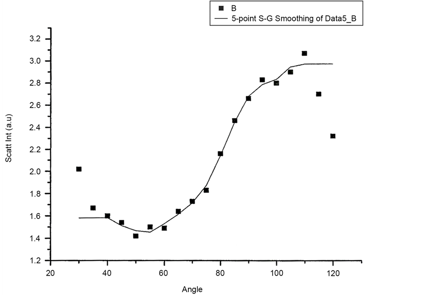
Figure 10. Scattered intensity vs angle for UNPOL-H configuration.
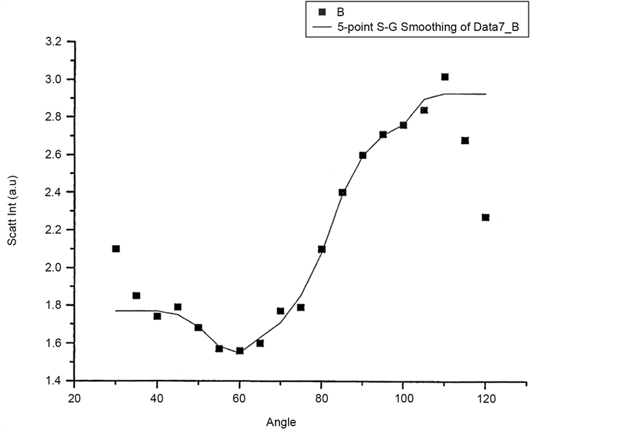
Figure 11. Scattered intensity vs angle for UNPOL-V configuration.
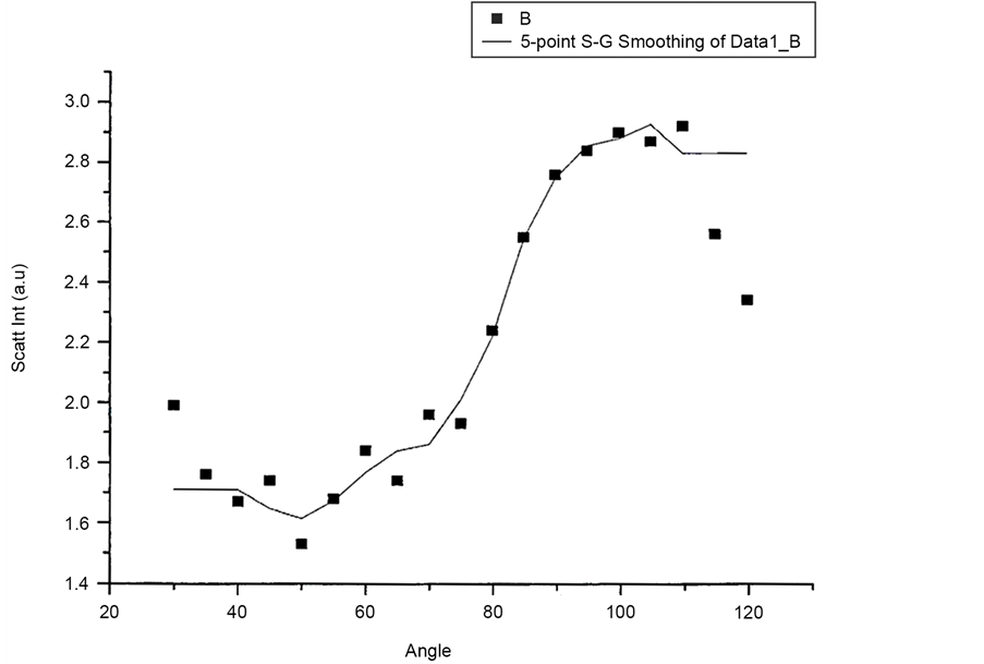
Figure 12. Scattered intensity vs angle for VH configuration.
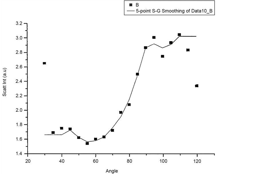
Figure 13. Scattering intensity vs angle for VV configuration.
 (a)
(a)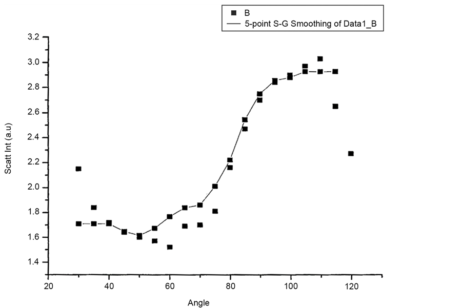 (b)
(b)
Figure 14. (a) Scattering intensity vs angle for CH configuration; (b) Scattering intensity vs angle for CV configuration.
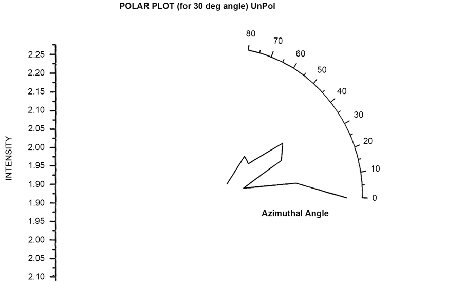
Figure 15. Scattered intensity vs azimuthal angle (at θ = 30 for unpolarized light).
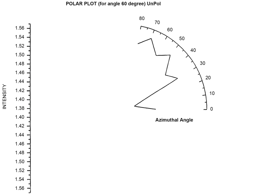
Figure 16. Scattered intensity vs azimuthal angle (at θ = 60 for unpolarized light).

Figure 17. Scattered intensity vs azimuthal angle (at θ = 90 for unpolarized light).
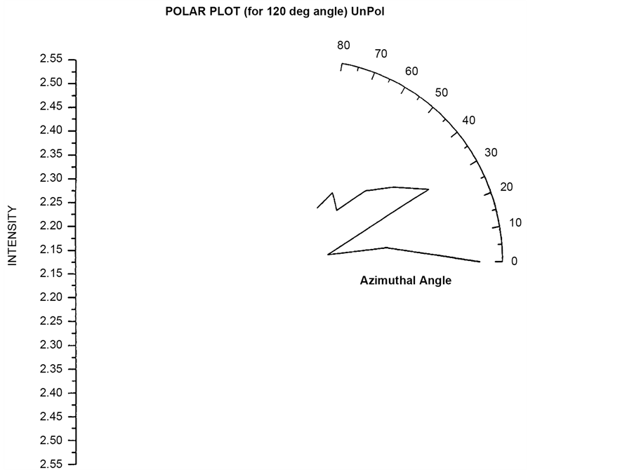
Figure 18. Scattered intensity vs azimuthal angle (at θ = 120 for unpolarized light).
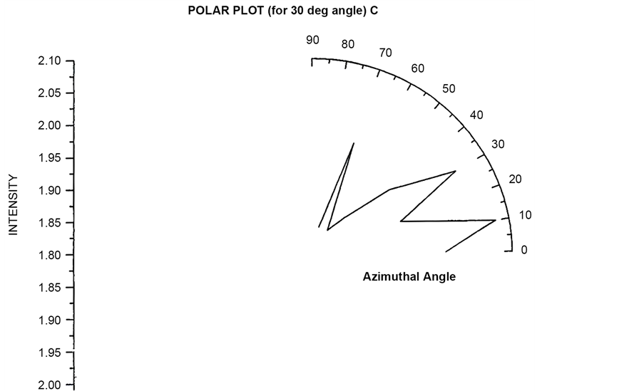
Figure 19. Scattered intensity vs azimuthal angle (at θ = 30 for circularly pol light).
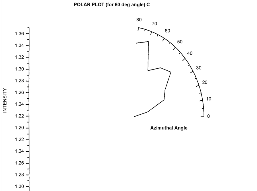
Figure 20. Scattered intensity vs azimuthal angle (at θ = 60 for circularly pol light).
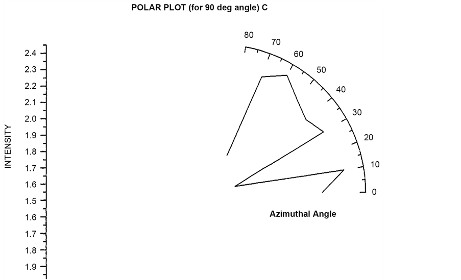
Figure 21. Scattered intensity vs azimuthal angle (at θ = 90 for circularly pol light).
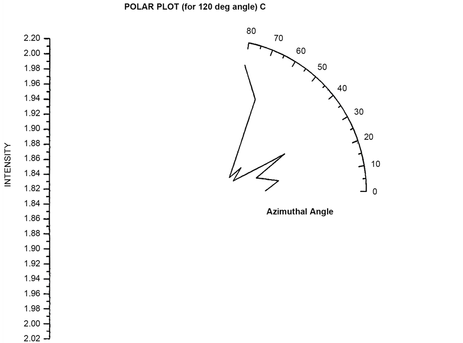
Figure 22. Scattered intensity vs azimuthal angle (at θ = 120 for circularly pol light).
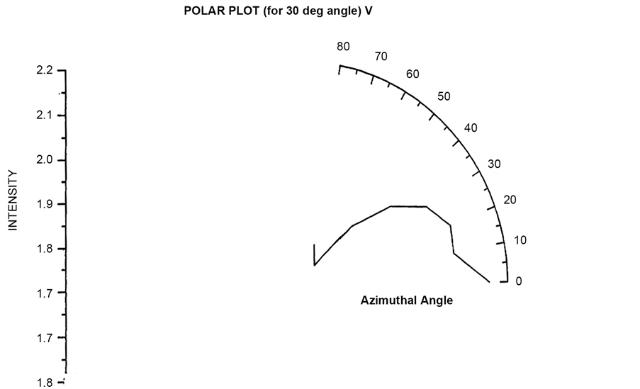
Figure 23. Scattered intensity vs azimuthal angle (at θ = 30 for vert pol light).
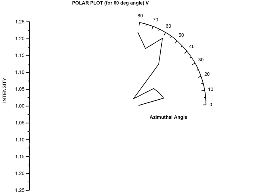
Figure 24. Scattered intensity vs azimuthal angle (at θ = 60 for vert pol light).

Figure 25. Scattered intensity vs azimuthal angle (at θ = 90 for vert pol light).
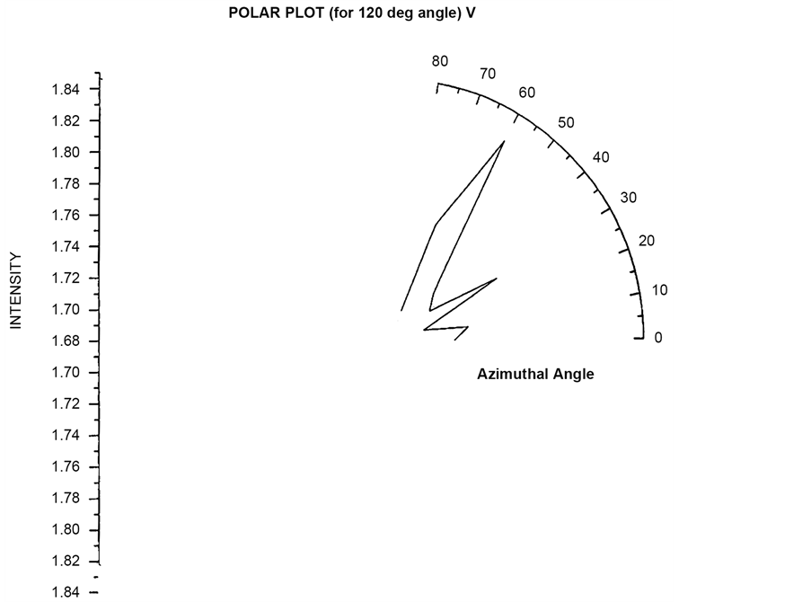
Figure 26. Scattered intensity vs azimuthal angle (at θ = 120 for vert pol light).
5. Conclusions
The present investigation is carried out to study the scattering properties of RBC cells with different polarized laser light as individual scatterrers. As it is evident from literature, RBC can form clusters or aggregates known as rouleuax. However, the present study is focused on single particle scattering from RBC which may be modeled as “disc shaped” particles. They can be studied as Mie scatterers. Nevertheless, the theory is formulated basically for spherical (larger) particles. RBC being discs can orient in many directions and to get insight into this phenomenon, we have plotted the polar plots. Polar plots with unpolarized, circular polarized and linear polarized incident light have been plotted. Scattered intensity Vs Angle shows similar angular variations for all polarization work.
Similar variation for polarization variations is seen in literature [30] [31] . Nevertheless, we do not expect clustering process in this study. It is expected that the plots are showing single particle scattering. Polar plots show predominant scattering at azimuthal angle φ = 30˚ & 60˚. But almost all plots show (Figures 15-26) predominant scattering in φ = 30˚. Bickel et al. have studied these scattering processes using scattering matrix formulation and has determined many of the scattering matrix elements [15] . Present study is oriented in this direction to study the effect of polarization states on the scattering matrix elements, although we have not gone into details.
The paper reports the fabrication of indigenously developed scattering spectrometer and it reports angle resolved scattered intensity plots. Also the Polar Plots have been plotted to show the significance of orientations. A quest of Ideal single particle scatters is underlying such experiment and theoretical studies.
Cite this paper
Joseph, D. and Kumar, A. (2016) Static Laser Light Scattering Studies from Red Blood Cells. Optics and Photonics Journal, 6, 237-260. http://dx.doi.org/10.4236/opj.2016.610025
References
- 1. Rayleigh, L. (1918) On Scattering of Light by Spherical Shells and by Complete Sphere of Periodic Structures. Proceedings of the Royal Society of London Series A, 94, 296-300.
http://dx.doi.org/10.1098/rspa.1918.0016 - 2. Stratton, J.A. (1941) Electromagnetic Theory. McGraw-Hill Book Co., New York.
- 3. Van de Hulst, H.C. (1957) Light Scattering from Small Particles. John Wiley & Sons Inc., New York.
- 4. Gans, R. (1925) Strahlungsdiagramme ultramikroskopischer Teilchen. Annals of Physics, 381, 29-38.
http://dx.doi.org/10.1002/andp.19253810103 - 5. Gans, R. (1912) über die Form ultramikroskopischer Goldteilchen. Annals of Physics, 342, 881-900.
http://dx.doi.org/10.1002/andp.19123420503 - 6. Mie, G. (1908) Beitrüge zur Optik trüber Medien, speziell kolloidaler Metallösungen. Annals of Physics, 330, 377-445.
http://dx.doi.org/10.1002/andp.19083300302 - 7. Hansen, J.P. and Hayter, J.B. (1982) A Rescaled MSA Structure Factor for Dilute Charged Colloidal Dispersions. Molecular Physics, 46, 65-656.
http://dx.doi.org/10.1080/00268978200101471 - 8. Sood, A.K. (1991) In: Ehrenreich, H. and Turnbull, D., Eds., Solid State Physics, Academic Press, Pittsburgh, 45, 1.
- 9. Copley, A.L. (1987) Clinical Hemerheology, 3-14.
- 10. Tuchin, V.V. (1997) Исследование биотканей методами светорассеяния. Uspekhi Fizicheskikh Nauk, 167, 517-539.
http://dx.doi.org/10.3367/UFNr.0167.199705c.0517 - 11. Tuchin, V.V. (2007) Tissue Optics: Light Scattering Methods and Instruments for Medical Diagnosis. SPIE Press, Bellingham.
http://dx.doi.org/10.1117/3.684093 - 12. Lugovtsov, A.E., Priezchev, A.V. and Yu, N.S. (2008) Proceeding of SPIE, 7022, 70220y-1.
- 13. Ranji, M., Jagard, D.L. and Chance, B. (2008) Observation of Mitochondrial Morphology and Biochemistry Changes Undergoing Apoptosis by Angularly Resolved Light Scattering and Cryoimaging. Proceeding of SPIE, 6087, Article ID: 60870K.
http://dx.doi.org/10.1117/12.646255 - 14. Alfano, R., Liang, X., Wang, L. and Ho, P.P. (1994) Time-Resolved Imaging of Translucent Droplets in Highly Scattering Turbid Media. Science, 264, 1913-1915.
http://dx.doi.org/10.1126/science.264.5167.1913 - 15. Bickel, W.S., Davidson, J.F., Huffman, D.R. and Kilkson, R. (1976) Time-Resolved Imaging of Translucent Droplets in Highly Scattering Turbid Media. Proceedings of the National Academy of Sciences of the United States of America, 73, 486-490.
http://dx.doi.org/10.1073/pnas.73.2.486 - 16. Lomakin, A., Teplow, D. and Benedek, G. (2005) Quasielastic Light Scattering for Protein Assembly Studies. In: Sigurdsson, E.M., Ed., Amyloid Proteins: Methods and Protocols, Humana Press Inc., Totowa, 299.
- 17. Park, M., Fu, D., Chai, P.G, Suresh, B. and Felt, M.S. (2010) Static and Dynamic Light Scattering of Healthy and Malaria-Parasite Invaded Red Blood Cells. Journal of Biomed Optics, 15, Article ID: 020506.
http://dx.doi.org/10.1117/1.3369966 - 18. Sorensen, C.M. and Lu, C.J. (1992) Test of Static Structure Factors for Describing Light Scattering from Fractal Soot Aggregates, Langmuir, 8, 2064-2069.
http://dx.doi.org/10.1021/la00044a029 - 19. Witten, T.A. and Sander, L.M. (1980) Diffusion-Limited Aggregation, a Kinetic Critical Phenomenon. Physical Review Letters, 47, 1400-1403.
http://dx.doi.org/10.1103/PhysRevLett.47.1400 - 20. Aubert, C. and Canell, D.S. (1986) Restructuring of Colloidal Silica Aggregates. Physical Review Letters, 56, 738-741.
http://dx.doi.org/10.1103/PhysRevLett.56.738 - 21. Ziff, R.F. (1984) In: Family, F. and Landau, D.P., Eds., Kinetics of Aggregation and Gelatin, Elsevier, Amsterdam.
- 22. Taflove, A. (1995) Computational Electrodynamics: The Finite Different Time Domain Method. Artech, Boston.
- 23. Waterman, P.C. (1971) Symmetry, Unitarity, and Geometry in Electromagnetic Scattering. Physical Review D, 3, 825-839.
http://dx.doi.org/10.1103/PhysRevD.3.825 - 24. Nilsson, A.M.K., Alsholm, P., Karlsson, A. and Andersson-Engels, S. (1998) T-Matrix Computations of Light Scattering by Red Blood Cells. Applied Optics, 37, 2735-2748.
http://dx.doi.org/10.1364/AO.37.002735 - 25. Barber, P.W. and Hill, S.C. (1990) Light Scattering by Particles: Computational Methods. World Scientific, Singapore.
http://dx.doi.org/10.1142/0784 - 26. Drain, B.T. and Flatau, J. (1994) Discrete-Dipole Approximation for Scattering Calculations. Optical Society of America A, 11, 1491-1499.
http://dx.doi.org/10.1364/JOSAA.11.001491 - 27. Draine B.T. (2000) In: Mishchenko, M.I., Hovenier, J.W. and Travis, L.D., Eds., Light Scattering by Nonspherical Particles: Theory, Measurements, and Applications, Academic Press, New York.
- 28. Tatarski, V.I. (1961) Wave Propagation in a Turbulent Medium. McGraw-Hill, New York.
- 29. Kak, A.C. and Slaney, M. (1988) Principal of Computerized Tomographic Imaging. IEEE Press, New York.
- 30. Lugovtsov, A.E., Priezzhev, A.V. and Yu, N.S. (2007) International Conference on Advanced Laser Technologies, Levi, 3-7 September 2007, 7022 0277-786X.
- 31. Shvalov, A.N., Soini, J.T., Chernyshev, A., Tarasov, P.A., Soini, E. and Maltsev, V.P. (1999) Light-Scattering Properties of Individual Erythrocytes. Applied Optics, 38, 230-235.
http://dx.doi.org/10.1364/AO.38.000230