Journal of Surface Engineered Materials and Advanced Technology
Vol.06 No.04(2016), Article ID:71169,15 pages
10.4236/jsemat.2016.64014
A Predictive Modeling Based on Regression and Artificial Neural Network Analysis of Laser Transformation Hardening for Cylindrical Steel Workpieces
Ahmed Ghazi Jerniti, Abderazzak El Ouafi, Noureddine Barka
Mathematics, Computer Science and Engineering Department, University of Quebec at Rimouski, Rimouski, Canada

Copyright © 2016 by authors and Scientific Research Publishing Inc.
This work is licensed under the Creative Commons Attribution International License (CC BY 4.0).
http://creativecommons.org/licenses/by/4.0/


Received: July 15, 2016; Accepted: October 9, 2016; Published: October 12, 2016
ABSTRACT
Laser surface hardening is a very promising hardening process for ferrous alloys where transformations occur during cooling after laser heating in the solid state. The characteristics of the hardened surface depend on the physicochemical properties of the material as well as the heating system parameters. To exploit the benefits presented by the laser hardening process, it is necessary to develop an integrated strategy to control the process parameters in order to produce desired hardened surface attributes without being forced to use the traditional and fastidious trial and error procedures. This study presents a comprehensive modelling approach for predicting the hardened surface physical and geometrical attributes. The laser surface transformation hardening of cylindrical AISI 4340 steel workpieces is modeled using the conventional regression equation method as well as artificial neural network method. The process parameters included in the study are laser power, beam scanning speed, and the workpiece rotational speed. The upper and the lower limits for each parameter are chosen considering the start of the transformation hardening and the maximum hardened zone without surface melting. The resulting models are able to predict the depths representing the maximum hardness zone, the hardness drop zone, and the overheated zone without martensite transformation. Because of its ability to model highly nonlinear problems, the ANN based model presents the best modelling results and can predict the hardness profile with good accuracy.
Keywords:
Heat Treatment, Laser Surface Hardening, Hardness Predictive Modeling, Regression Analysis, Artificial Neural Network, Cylindrical Steel Workpieces, AISI 4340 Steel, Nd:Yag Laser System

1. Introduction
AISI 4340 is a nickel-chromium-molybdenum alloy steel known for its toughness and its ability to attain high strengths when heat-treated, while retaining good fatigue strength. Typical applications are for structural use, such as aircraft landing gear, power transmission gears and shafts and other structural parts. This alloy may be heat treated to high strength levels while maintaining good toughness, wear resistance and fatigue strength levels, as well as good atmospheric corrosion resistance [1] .
When compared with conventional hardening methods such as oven, flame, or induction hardening, laser hardening is marked by a range of advantages such as spatially and temporally limited energy deposition, which eliminates the need for quenching with water, oil, or salt baths. Laser hardening allows for a highly defined zone of influence without affecting neighboring surfaces, and high cooling rates make fine structures and high levels of hardness possible. Intricate contours are easily hardened using lasers due to the flexible beam guidance possibilities, also making it possible to harden parts directly where it is required [2] .
In surface hardening using laser radiation, carbonic steel is heated above the austenization temperature for a short time. Through rapid cooling the steel reaches the martensitic material structure. Heat deposition is realized through the absorption of laser radiation at the surface of the material, whereas cooling occurs conductively within the remaining material [3] .
There are many methods for modeling the laser hardening process, such as the finite element method (FE), the regression method, and the artificial neural network method (ANN). The principle of the FE method is solving the heat transfer differential equation to determine the evolution of the studied workpiece temperature versus time; the maximum temperature and cooling rate on the surface of the workpiece are calculated to determine the hardened zone. Many researchers used this method for plate [4] - [6] and cylindrical shaped [7] - [10] workpieces forms. Regression modeling is an empirical modeling technique derived for the evaluation of the relationship of a set of controlled experimental factors and observed results. This method is used in several cases [11] - [13] to model and understand the effect of laser hardening parameters on several hardened zone properties.
The laser heat treatment of cylindrical pieces is done with a combination of two movements: a rectilinear movement of the articulated robot carrying the laser fiber, and a rotation of the cylindrical part generated by a DC motor. This combination of two speeds during treatment makes the finite element model simulation slower and difficult to calibrate, which leads us to choose ANN modeling methods. This is a powerful modeling tool that has the ability to identify complex relationships from data for nonlinear problems compared to regression modeling, despite the significant number of experimental tests required for the modeling.
Research based on ANN modeling for laser hardening on cylindrical workpieces is not numerous. In the literature there is one conference paper [14] presenting a model for the prediction of the laser surface hardening index on a cylinder liner based on a radial basis function neural network prediction model. The processes parameters are laser power (250 W - 350 W), scanning speed (20 mm/s - 30 mm/s), and spot diameter size (1 mm - 2 mm). Despite its ability of surface hardness and hardened depth prediction, the ANN model includes a limited scale of process parameter variation and is not able to predict the heat affected zone, which has a drop in initial hardness.
2. Experimental Setup
The experimentations are performed by using a commercial 3 kW Nd:Yag laser source (IPG YLS-3000-ST2) combined with a 6 degrees of freedom articulated robot. This type of laser generates a beam with a wavelength λ = 1064 µm. The AISI 4340 steel cylindrical parts, with 18 mm diameter 50 mm length, are mounted on a lathe as illustrated in Figure 1. All of the parts used were oven heated and oil quenched and then oven tempered before laser hardening at the same time and under the same conditions; this preprocessing produces the same hardness in all parts and blackens their surface areas to increase laser surface absorption. The hardness of the workpieces after the oven heat treatment operations is about 44-46HRC.
A rotating testing rig is used during this experiment to rotate the workpieces throughout the laser heat treatment, and the laser beam is set to point the median plane of the cylinder, and remain in it during the translation motion of the articulated robot. The cooling of the workpieces is done by radiation and conduction without any external cooling source. After the laser transformation hardening, the specimens were cut perpendicularly to the cylinder’s axis of revolution, and the required surface of each specimen was ground and polished with various grades of emery sheets. The hardened zone characteristics are determined by the surface hardness profile. Hardness measurements were done from the surface to the center of the workpiece, using Vickers’s tests with a load of 300 g applied for 15 s. For each trial, different hardness profiles with 50 μm steps were measured.
The process parameters in this article are the laser power (LP), the scanning speed (SS) of the laser beam, and the revolution speed (RS) of the part. Preliminary tests allow
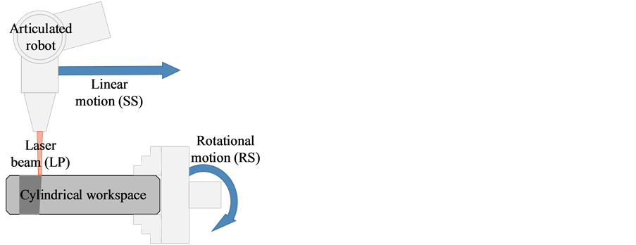
Figure 1. Experimental setup.
the determination of process parameter limits so the non-hardening or melting of the workpieces can be avoided. Ranges of 1800 W to 2400 W laser power (LP), and 3 mm/s to 6 mm/s scanning speed (SS) allow the heat treatment of parts without producing melting or hardening discontinuity. The revolution speed is limited on the upper end by the limits of the DC motor rotating the workpieces, and on the lower end by the regularity of the hardened zone, so a range of 3000 rpm to 6000 rpm is used in the test matrix.
Due to its simplicity and transparency, a systematic design based on the factorial design is the most commonly used model in experimentation. However, this requires a substantial number of tests depending on the number of factors and their levels. In this way, the use of a testing strategy such as the orthogonal arrays developed by Taguchi leads to an efficient and robust fractional factorial design of experiments that can collect all the statistically significant data with a minimum number of repetitions [15] . Accordingly, in this paper an L16 Taguchi test matrix is used for the modeling the process. The L16 illustration the mixture parameters used for regression and artificial neural networks modeling and analysis is presented in detail in Table 1.
An L9 Taguchi test matrix composed of central tests of L16 Taguchi matrix is used to validate the model is presented in Table 2. The central test (2100 W for LP, 4.5 mm/s for SS, and 4500 rpm for RS) is repeated 10 times (called R1 to R10 in the rest of the paper) in order to evaluate the process repeatability and the errors of measurement.

Table 1. L16 Taguchi test matrix.
Table 2. L9 Taguchi test matrix.
The hardness curve obtained by laser heat treatment is illustrated in Figure 2. The first region (zone1) is characterized by the maximum hardness of the curve; it is completely transformed to austenitic phase during the heating process and then to martensitic structure upon quick cooling. The second region (zone2) represents the hardness loss caused by sharp drop in hardness to reach a minimum value, representing a rise in hardness until it reaches the initial hardness value. This zone is heated by using a temperature between the start temperature of austenitisation, giving overtempered martensite after cooling (H2 hardness), and the temperature of complete autenitisation, giving hard martensite after cooling (H1 hardness). The third region (zone3) is heated enough, but without reaching the austenite formation start temperature; therefore it is completely tempered by the heat flow effect, which is stronger in the area closest to the surface of the workpiece. Finally, the fourth region (zone4) corresponds to the zone unaffected by the thermal flow [16] .
The effects of different laser hardening parameters are determined using the hardness curve, which is characterized by identifying boundary points for the four different areas: D1 and H1 for the zone1/zone2 limit, D2 and H2 for the zone2/zone3 limit, and D3 and H3 for the zone3/zone4 limit. Throughout the article D1, D2 and D3 are expressed in µm, and H1 and H2 are expressed in HRC. H3 represents the initial hardness of the workpieces, and is fixed at 44HRC to determine D3.
The repeatability test is made to assess the robustness and reproducibility of the process, as well as errors resulting from measurement steps (50 µm between every two measurements of the microhardness) and shift of the measurement position. The central test of the validation table (2100 W for LP, 4.5 mm/s for SS, and 4500 rpm for RS) is repeated 10 times. Table 3 shows the results of the repeatability of the 10 tests and statistical calculations (the average value, the standard deviation, and the gap between the maximum and the minimum).
Table 3. The results of the repeatability tests.

Figure 2. Typical curve of surface hardness profile obtained by laser hardening of AISI 434 steel.
The gap between the maximum and the minimum hardness value of all the modeling and the validation data is 4.15HRC for H1 and 2.28HRC for H2, while the gap representing the repeatability and the measurement errors determined by the repeatability study is 1.47HRC for H1 and 1.25HRC for H2, which represents an error of 35% for H1 and 55% for H2. This is caused by the fact that the cooling rate, which is not controlled in the present work, is highly affecting the hardening process. On the other hand the gap between the maximum and the minimum depths values of the modeling and the validation data is 382.7 µm for D1, 490.3 µm for D2, and 1441.3 µm for D3, while the gap representing the repeatability and the measurement errors determined by the repeatability study is 11.3 µm for D1, 12.6 µm for D2, and 75.5 µm for D3, which represents an error of 2.9% for D1, 2.6% for D2, and 5.2% for D3. The error is low because these depths depend on the maximum temperature reached by heating and not the cooling rate [17] , thus only D1, D2, and D3 are considered in the following. Table 4 regroups all of the results of the modeling tests (M1 to M16) and the validation tests (V1 to V9).
3. Regression Model
The analysis of variance aims to study the effects of different parameters on the hardness profile. It gives the contribution of each parameter in the variation of process parameters. Table 5 shows the detailed ANOVA of the depths (D1, D2, and D3). The most significant parameter is the scanning speed (SS), its contribution is about 69% for D1 and D2, and more than 81% for D3. Laser power (LP) is also an important parameter with a contribution of more than 22% for D1 and D2, and about 15% for D3. The revolution speed has a contribution of less than 5% for D1 and D3, and less than 1% for D3, so its effect is neglected for D3. The error for all the depths is less than 4%, which means that all the significant parameters of the process are considered.
Figure 3 shows the effect of all parameters on the depths (D1, D2, and D3). These depths increase with increasing the laser power and decrease with decreasing scanning speed and revolution speed. The graphs also confirm the ANOVA results. The objective is to predict the depths (D1, D2, and D3) with the given process parameters provided by modeling data (M1 − M16), and validate the regression model with the validation data


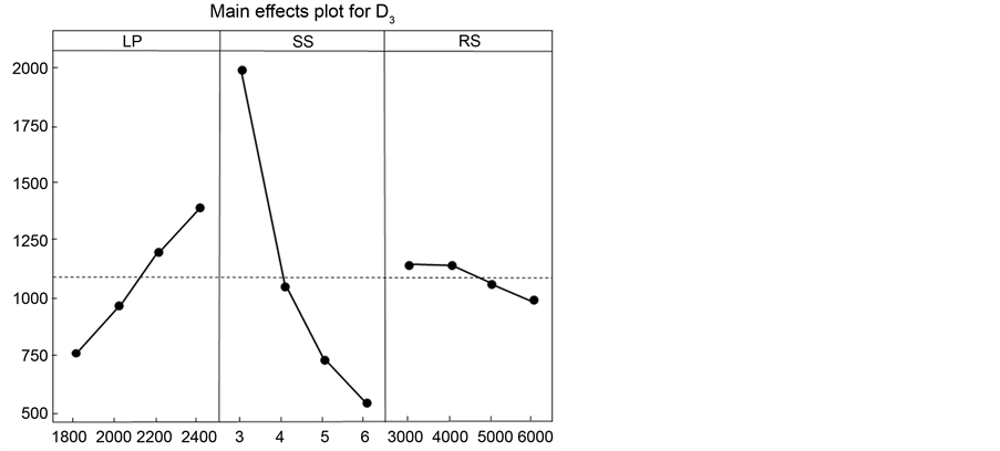
Figure 3. Effects of laser power, scanning speed, and revolution speed on D1, D2 and D3.
Table 4. The results of the modeling and validation tests.
Table 5. ANOVA table for D1, D2 and D3.
(V1 − V9). The empirical relationship between the depths (D1, D2, and D3) and the laser process parameters can be expressed by Equations (1)-(3), which presents a model based on fit regression modeling and allows the evaluation of the depths (D1, D2, and D3) as a function of the laser parameters (LP, SS, and RS).


Figure 4 shows the depths (D1, D2, and D3) calculated using the regression formula (Equations (1)-(3)) for all 16 modeling data points and the 9 validation data points of the process parameters, and their distribution around the bisector of the quadrant. The mean relative error is 10.5% for D1, 9.1% for D2, and 7.9% for D3 between the depths calculated with the regression formula and the experimental ones; the coefficient of determination, R2, is 0.9830 for D1, 0.9828 for D2, and 0.9726 for D2. The maximum relative error is still important, thus neural network modeling is proposed in the following chapter.
4. Artificial Neural Networks Model
ANNs are relatively new computational tools that have found extensive utilization in solving many complex problems. The attractiveness of ANNs comes from their
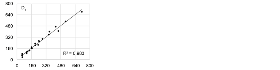


Figure 4. Scatter plot-measured and predicted D1, D2 and D3 using the regression model.
remarkable information processing characteristics, pertinent mainly to nonlinearity, fault and noise tolerance, and learning and generalization capabilities. The idea of ANNs is not to replicate the operation of the biological system, but to make use of what is known about the functionality of biological networks for solving complex problems. ANN models are empirical, however, they can provide practically accurate solutions for precisely or imprecisely formulated problems and for phenomena recorded as field observations. These models learn from the preceding data obtained, which is named the training set, and then check the system accomplishment using test data [18] .
The basic units of ANNs are neurons, which are connected to each other with a weight factor. ANNs are networks of highly interconnected neural computing elements that have the ability to respond to input stimuli and to learn to adapt to the environment. While a single-layer network has single input or output units, a multilayer network has one or more hiding units between the input and output layers. The multilayer perceptron consists of a system of simple interconnected neurons, or nodes, as illustrated in Figure 5, representing a nonlinear mapping between inputs and outputs. The nodes are connected by weights and output signals, which are a function of the sum of the inputs to the node, modified by a simple nonlinear function. Two working phases are included in ANN models: the phase of learning and the phase of recall. During the learning phase, known data sets are commonly used as a training signal in input and output layers. The recall phase is performed in one run using the weights obtained during the learning phase [19] .
The choice of the best ANN structure for modeling a given process is done by varying the number of hidden layers and the number of neurons in each one. Each ANN structure is trained several times to avoid the effect of the randomly chosen weight coefficients in the beginning of the learning phase. The first trial of ANN modeling was done with one hidden layer, and the number of neurons in the hidden layer was varied. Results show that the learning becomes perfect for over 20 neurons, but the model cannot be validated with the validation data. For less than 20 neurons the model has a high gap between prediction and experimentation, therefore the use of several hidden layers is beneficial. The number of neurons in each hidden layer is varied from 1 to 20, and the best model is found to have a neural structure of 3 neurons in the input layer (LP, SS, and RS), three hidden layers having the structure 2-15-8, and an output layer of 3 neurons (D1, D2, and D3). This model has a coefficient of determination, R2, of 1.000 for the modeling data and 0.995 for the validation data. The average error for all the modeling and validation data is 3.5% for D1, 2.2% for D2, and 2.5% for D3; the maximum relative error is 12.6% for D1, 13.1% for D2, and 10.7% for D3; and the gap between the maximum error and the minimum error is 46.7 µm for D1, 42.8 µm for D2, and 150.8 µm for D3.
Figure 6 shows the depths (D1, D2, and D3) predicted by the ANN model for all 16 modeling data points and the 9 validation data points for process parameters and their distribution around the bisector of the quadrant. The coefficient of determination is 0.9969 for D1, 0.9985 for D2, and 0.9968 for D3. All the points are on the bisector, which

Figure 5. The ANN based model structure.


Figure 6. Scatter plot-measured and predicted D1, D2 and D3 using the ANN based model.
means that the model is perfectly accurate compared to the regression model.
Using the modeling and validation tests, the fitness of the ANN model and the regression model (R-model) are characterised in Table 6. The regression squared value is used for the modeling data (RM2) and the validation data (RV2) for all depths, as well as for the depths separately (RD12, RD22, and RD32) using modeling and validation data. Also shown is the average error for all depths, and the margin of error which represents the gap between the maximum and the minimum model errors divided by the median for each response (D1-3).
The ANN based model is much better than the regression based model, as shown in Table 6, in terms of the regression squared and the average errors expressed as a percentage. The gaps between the maximum and minimum error in the ANN model are 46.7 µm for D1, 42.8 µm for D2, and 150.8 µm for D3, and the gaps in error for the regression model are 44.7 µm for D1, 65.9 µm for D2, and 247.9 µm for D3. These errors represent the errors of the model, the errors produced by process repeatability, and the errors of measurement, which was determined previously to be 11.3 µm for D1, 12.6 µm for D2, and 75.7 µm for D3. These measurement errors of and repeatability errors represent noise in the modeling process, which ANN modeling clearly demonstrates its ability to avoid.
Figure 7 shows a comparison between the hardness curves obtained by microhardness measurements, the curve shape predicted by the regression model, and the curve shape predicted by the ANN model for the validation testes V2, V4, V6, and V8. The graphs shows that both models are able to predict the microhardness curve shape, with the ANN model closest to reality.
5. Conclusion
In this paper, a predictive modeling based on regression and artificial neural network analysis of laser transformation hardening for cylindrical of AISI 4340 steel workpieces is presented. Several laser surface transformation hardening parameters and conditions are analyzed and their correlation with multiple physical and geometrical attributes is examined using a structured experimental and numerical modelling investigations under consistent practical process conditions. After identifying the parameters that provide the best information about the laser heating and the surface transformation process, conventional regression and artificial neural network analysis are proposed to build an accurate and consistent hardness profile prediction model. The process parameters included in the study are laser power, beam scanning speed, and the workpieces rotational speed. The upper and the lower limits for each parameter are chosen considering the start of the trans-formation hardening and the maximum hardened zone without surface melting (1800 W to 2400 W for the laser power, 3 mm/s to 6 mm/s for the scanning speed, and 3000 rpm to 6000 rpm for the workpiece rotational speed). The
Table 6. The regression squared, average error and gap for the regression model and the ANN based model.

Figure 7. Comparison between measurement and prediction models for tests V2, V4, V6 and V8.
hardened surface physical and geometrical attributes are extracted from the experimental microhardness curves. The results demonstrate that the resulting models are able to predict the depths representing the maximum hardness zone, the hardness drop zone and the overheated zone without martensite transformation. Because of its ability to model highly nonlinear problems, the artificial neural network based predictive model presents the best results and can predict the hardness profile with good accuracy. Globally, the performance of the hardness profile prediction model shows significant improvement. With a global maximum relative error less than 5% under various conditions, the prediction model can be considered efficient and have led to conclusive results, due to the complexity of the heat treatment process. The performance of the modelling process can be improved by including additional surface transformation hardening parameters and conditions. The inclusion of parameters like surface roughness and cooling rate in the predictive modelling procedures with others applications for complex geometric features are among the main directions to consider for the future works.
Cite this paper
Jerniti, A.G., El Ouafi, A. and Barka, N. (2016) A Predictive Modeling Based on Regression and Artificial Neural Network Analysis of Laser Transformation Hardening for Cylindrical Steel Workpieces. Journal of Surface Engineered Materials and Advanced Technology, 6, 149-163. http://dx.doi.org/10.4236/jsemat.2016.64014
References
- 1. Miracle, D.B., Donaldson, S.L., Henry, S.D., Moosbrugger, C., Anton, G.J., Sanders, B.R., Hrivnak, N., Terman, C., Kinson, J. and Muldoon, K. (2001) ASM Handbook. ASM international Materials Park, OH, USA.
- 2. Migliore, L.R. (1996) Laser Materials Processing. CRC Press, Marcel Dekker, New York.
- 3. Kennedy, E., Byrne, G. and Collins, D. (2004) A Review of the Use of High Power Diode Lasers in Surface Hardening. Journal of Materials Processing Technology, 155, 1855-1860.
http://dx.doi.org/10.1016/j.jmatprotec.2004.04.276 - 4. Wu, W., Liang, N., Gan, C. and Yu, G. (2006) Numerical Investigation on Laser Transformation Hardening with Different Temporal Pulse Shapes. Surface and Coatings Technology, 200, 2686-2694.
http://dx.doi.org/10.1016/j.surfcoat.2004.11.011 - 5. Shuja, S. and Yilbas, B. (2013) Laser Multi-Beam Heating of Moving Steel Sheet: Thermal Stress Analysis. Optics and Lasers in Engineering, 51, 446-452.
http://dx.doi.org/10.1016/j.optlaseng.2012.11.006 - 6. Li, R., Jin, Y., Li, Z. and Qi, K. (2014) A Comparative Study of High-Power Diode Laser and CO2 Laser Surface Hardening of AISI 1045 Steel. Journal of Materials Engineering and Performance, 23, 3085-3091.
http://dx.doi.org/10.1007/s11665-014-1146-x - 7. Skvarenina, S. and Shin, Y.C. (2006) Predictive Modeling and Experimental Results for Laser Hardening of AISI 1536 Steel with Complex Geometric Features by a High Power Diode Laser. Surface and Coatings Technology, 201, 2256-2269.
http://dx.doi.org/10.1016/j.surfcoat.2006.03.039 - 8. Patwa, R. and Shin, Y.C. (2007) Predictive Modeling of Laser Hardening of AISI5150H Steels. International Journal of Machine Tools and Manufacture, 47, 307-320.
http://dx.doi.org/10.1016/j.ijmachtools.2006.03.016 - 9. Giorleo, L., Ceretti, E. and Giardini, C. (2013) Fe Modeling of the Apparent Spot Technique in Circular Laser Hardening. The International Journal of Advanced Manufacturing Technology, 69, 1961-1969.
http://dx.doi.org/10.1007/s00170-013-5162-z - 10. Orazi, L., Liverani, E., Ascari, A., Fortunato, A. and Tomesani, L. (2014) Laser Surface Hardening of Large Cylindrical Components Utilizing Ring Spot Geometry. CIRP Annals— Manufacturing Technology, 63, 233-236.
http://dx.doi.org/10.1016/j.cirp.2014.03.052 - 11. Babu, P.D., Buvanashekaran, G. and Balasubramanian, K. (2013) Experimental Investigation of Laser Transformation Hardening of Low Alloy Steel Using Response Surface Methodology. The International Journal of Advanced Manufacturing Technology, 67, 1883- 1897.
http://dx.doi.org/10.1007/s00170-012-4616-z - 12. El-Batahgy, A.-M., Ramadan, R.A. and Moussa, A.-R. (2013) Laser Surface Hardening of Tool Steels—Experimental and Numerical Analysis. Journal of Surface Engineered Materials and Advanced Technology, 3, 146-153.
http://dx.doi.org/10.4236/jsemat.2013.32019 - 13. Barka, N. and El Ouafi, A. (2015) Effects of Laser Hardening Process Parameters on Case Depth of 4340 Steel Cylindrical Specimen—A Statistical Analysis. Journal of Surface Engineered Materials and Advanced Technology, 5, 124-135.
http://dx.doi.org/10.4236/jsemat.2015.53014 - 14. Wu, X.L. and Ren, F. (2011) Research on the Prediction Model of Laser Surface Hardening Index on Cylinder Liner Based on RBF. Advanced Materials Research, 148-149, 215-218.
http://dx.doi.org/10.4028/www.scientific.net/AMR.368-373.215 - 15. Ross, P.J. (1996) Taguchi Techniques for Quality Engineering: Loss Function, Orthogonal Experiments, Parameter and Tolerance Design. 2nd Edition, McGraw-Hill, New York.
- 16. Shiue, R. and Chen, C. (1992) Laser Transformation Hardening of Tempered 4340 Steel. Metallurgical Transactions A, 23, 163-170.
http://dx.doi.org/10.1007/BF02660862 - 17. Ashby, M. and Easterling, K.E. (1984) The Transformation Hardening of Steel Surfaces by Laser Beams—I. Hypo-Eutectoid Steels. Acta Metallurgica, 32, 1935-1948.
http://dx.doi.org/10.1016/0001-6160(84)90175-5 - 18. Zhang, H.C. and Huang, S.H. (1995) Applications of Neural Networks in Manufacturing: A State-of-the-Art Survey. International Journal of Production Research, 33, 705-728.
http://dx.doi.org/10.1080/00207549508930175 - 19. Rafiq, M., Bugmann, G. and Easterbrook, D. (2001) Neural Network Design for Engineering Applications. Computers & Structures, 79, 1541-1552.
http://dx.doi.org/10.1016/S0045-7949(01)00039-6