American Journal of Computational Mathematics
Vol.2 No.3(2012), Article ID:23155,10 pages DOI:10.4236/ajcm.2012.23022
A Generalized FDTD Method with Absorbing Boundary Condition for Solving a Time-Dependent Linear Schrödinger Equation
1Department of Physics, Louisiana Tech University, Ruston, USA
2Department of Mathematics & Statistics, Louisiana Tech University, Ruston, USA
Email: dai@coes.latech.edu
Received April 17, 2012; revised June 19, 2012; accepted June 27, 2012
Keywords: Schrodinger Equation; Absorbing Boundary; FDTD Method; Stability
ABSTRACT
The Finite-Difference Time-Domain (FDTD) method is a well-known technique for the analysis of quantum devices. It solves a discretized Schrödinger equation in an iterative process. However, the method provides only a second-order accurate numerical solution and requires that the spatial grid size and time step should satisfy a very restricted condition in order to prevent the numerical solution from diverging. In this article, we present a generalized FDTD method with absorbing boundary condition for solving the one-dimensional (1D) time-dependent Schrödinger equation and obtain a more relaxed condition for stability. The generalized FDTD scheme is tested by simulating a particle moving in free space and then hitting an energy potential. Numerical results coincide with those obtained based on the theoretical analysis.
1. Introduction
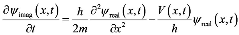
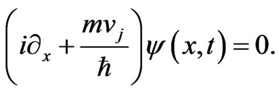
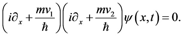
The 1D time-dependent linear Schrödinger equation, which is the basis of quantum mechanics [1,2], can be expressed as follows [3,4]:
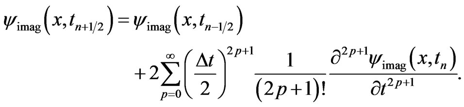
 , (1)
, (1)
where m is the mass of the particle (kg),  J·sec is Planck’s constant, V is the potential (J),
  is a complex number, and
  The product of
  with its complex conjugate,
  indicates the probability of a particle being at spatial location x at time t.
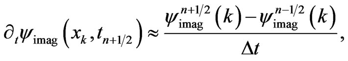
It can be easily seen that the classic explicit two-level in time finite difference scheme, i.e.,
 , (2)
, (2)
is unconditionally unstable, where  is the approximation of
 . Here,
  and
and  are the spatial grid size and time step, respectively,
  that denotes the set of all positive and negative integers, and
  is a second-order central difference operator such that
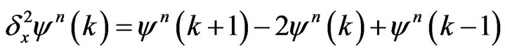 . (3)
. (3)
There are many numerical schemes developed for solving linear Schrödinger equations [1-33]. In particular, Sullivan [3] and Visscher [4] applied the finite-difference time-domain (FDTD) method, which is often employed in simulations of electromagnetic fields, to solve the above Schrödinger equation. The application of FDTD technique for the analysis of quantum devices is often called the FDTD-Q scheme, which can be described as follows [3].
The variable  is first split into its real and imaginary components in order to avoid using complex numbers:
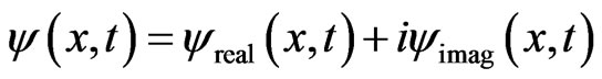 . (4)
. (4)
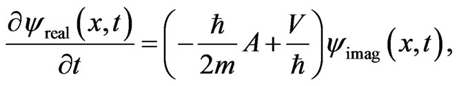
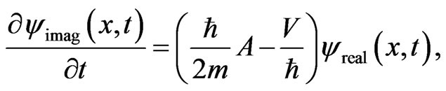
Inserting Equation (4) into Equation (1) and then separating the real and imaginary parts result in the following coupled set of equations:
 ,(5)
,(5)
and
 . (6)
. (6)
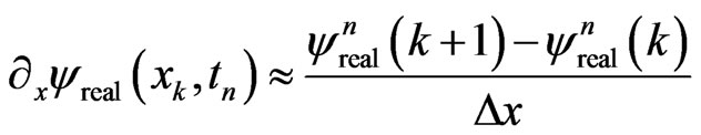
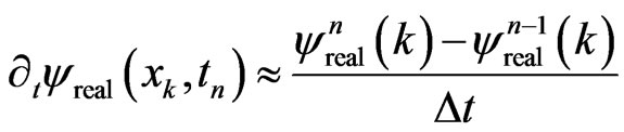
Thus, the second-order central finite difference approximations in space and time result in the FDTD-Q schemes as follows:
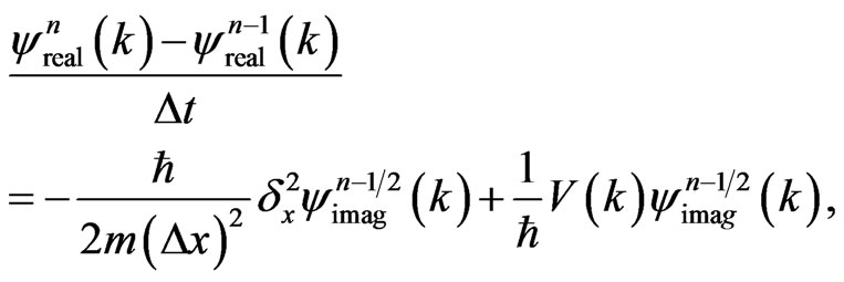 (7)
(7)
and
 (8)
(8)
Here, we assume that V is dependent only on x for simplicity. The computation of the above FDTD-Q scheme is very simple and straight-forward because one may obtain  from Equation (7) and then
  from Equation (8). Previously, the second author analyzed the stability of the FDTD-Q scheme using the discrete energy method and obtained a condition for determining the time step,
  , so that the scheme is stable as follows [13]:
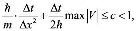 (9)
(9)
where c is a constant. It should be pointed out that Soriano et al. [27] and Visscher [4] also used the eigenvalue method to analyze the stability of the FDTD-Q scheme and obtained a very similar condition of
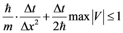 However, as pointed out in [13], even if the condition
 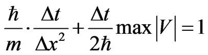 is chosenthe numerical solution is still divergent. Equation (9) indicates that the condition must be less than 1 but not close to 1.
The motivation of this study is to apply the idea of the FDTD method to develop a generalized FDTD method with absorbing boundary condition for solving the linear Schrödinger equation, so that a more relaxed condition for stability may be obtained.
2. Generalized FDTD Method
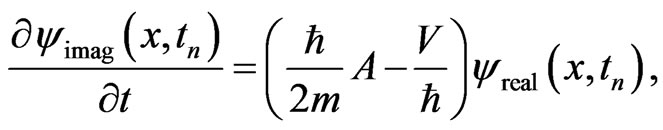
To develop a generalized FDTD scheme, we assume that 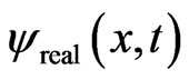 and
and  are sufficiently smooth functions which vanish for sufficiently large
  and the potential V is dependent only on x. We first rewrite Equations (5) and (6) as
 (10)
(10)
 (11)
(11)
where 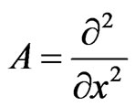 and employ the Taylor series method to expand
  and
and  at
at  as follows:
 (12)
(12)
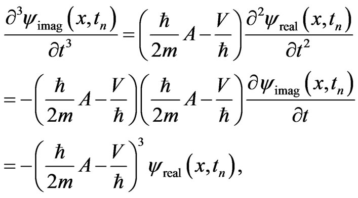
We then evaluate those derivatives in Equation (12) by using Equations (10) and (11) repeatedly:
 (13a)
(13a)
 (13b)
(13b)
 (13c)
(13c)
and so on. Substituting Equation (13) into Equation (12) gives
 (14)
(14)
Similarly, we employ the Taylor series method to expand  and
and  at
at  as follows:
 (15)
(15)
Again, using Equations (10) and (11) repeatedly to evaluate those derivatives in Equation (15), we obtain
 (16a)
(16a)
 (16b)
(16b)
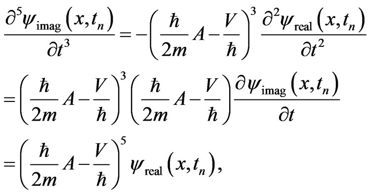 (16c)
(16c)
and so on. Substituting Equation (16) into Equation (15) gives
 (17)
(17)
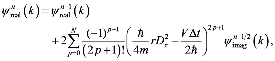
Thus, if 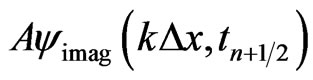 and
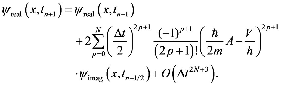
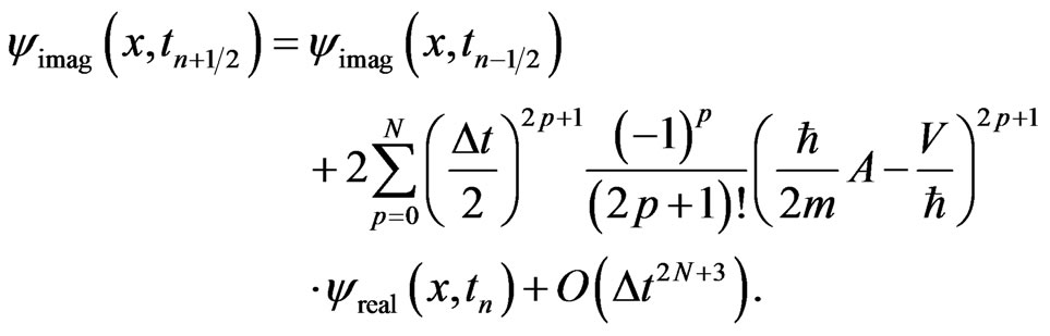
and 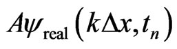 are approximated using some accurate finite differences, one may obtain a generalized FDTD scheme for solving the time-dependent linear Schrödinger equation as follows:
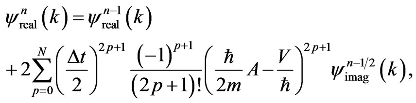 (18a)
(18a)
 (18b)
(18b)
It should be pointed out that in Equation (18a)  may be approximated by a higher-order accurate Lagrange polynomial or some other higher-order accurate approximations. Once
  is obtained from Equation (18a), one may construct a similar higherorder accurate Lagrange polynomial or some other higher-order accurate approximations for
  and then substitute it into Equation (18b) to obtain
 . Here, for simplicity, we limit ourselves to using finite difference approximations for the Laplace operator A. Furthermore, it can be seen from the above derivations that Equation (18) can be readily generalized to the multi-dimensional cases. For the case where the potential V is dependent on both temporal and spatial variables, the derivations are similar to those in Equation (16) except that the product rule of derivative with respect to t should be used.
3. Stability
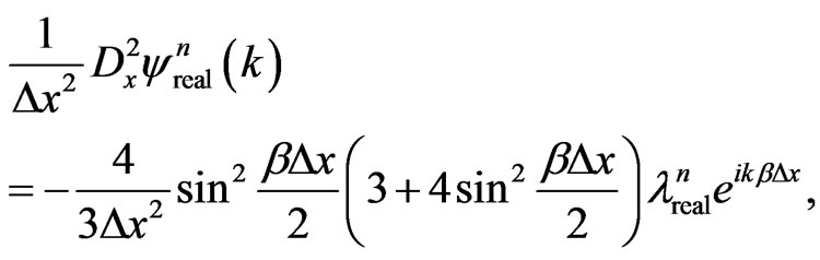
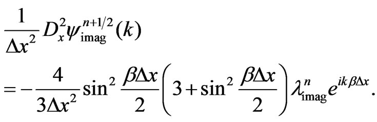
In order to prevent the numerical solution from diverging, we need to analyze the stability of the generalized FDTD method in Equation (18). Here, we consider that the Laplace operator A is only approximated by either a second-order central difference operator 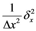 or a fourth-order central difference operator
 , where
 (19a)
(19a)
 (19b)
(19b)
and similar finite difference approximations for  . We assume that V is a constant and use the Von Neumann analysis [34] to analyze the stability of the generalized FDTD schemes. To this end, we first let
  and
and 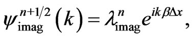 where
where  and
and  are amplification factors for
  and
and , respectively, and substitute them into Equation (19a). This gives
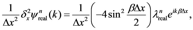 (20a)
(20a)
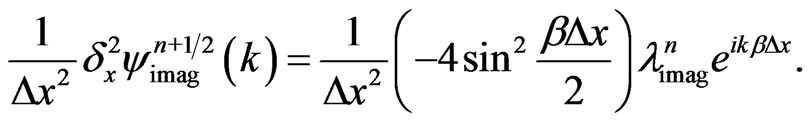 (20b)
(20b)
Replacing A with  in Equation (18), substituting Equation (20) into the resulting equations, and then deleting the common factor
 , we obtain
 (21a)
(21a)
 (21b)
(21b)
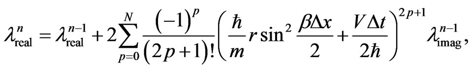
where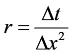 . Since Equation (21a) is true for any time level n, we rewrite Equation (21a) as
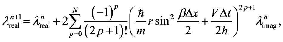 (22)
(22)
substract it by Equation (21a), and then use Equation (21b) to eliminate . As such, we obtain a quadratic equation for
  as follows:
 (23)
(23)
where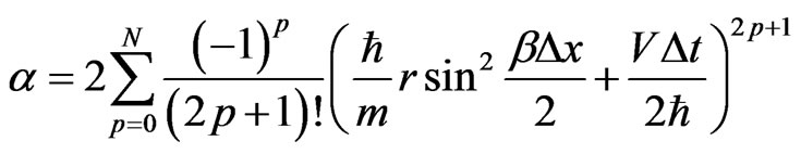 , Using the fact that for a quadratic equation
 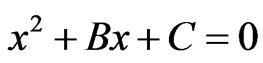 the solution x satisfies
  if and only if
 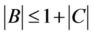 and
and 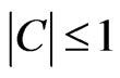 we obtain from Equation (23) that
 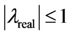 if and only if
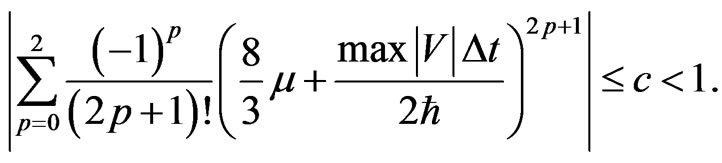
 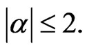 By the Von Neumann analysis, we conclude that the generalized FDTD scheme is stable if
 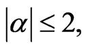 i.e.,
i.e.,
 (24)
(24)
It can be seen that
 (25)
(25)
implying that, when  Equation (24) is automatically satisfied, and, hence, the scheme with
 , is unconditionally stable. However, we cannot choose
  and, therefore, the generalized FDTD scheme should be imposed the condition in Equation (24). Noting that the condition in Equation (24) gives only
  and does not indicate whether or not there is a double root with
 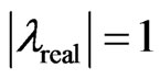 in Equation (23) (for this case, the numerical solution may still blow up), we choose the
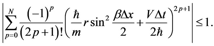
maximum value of 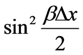 and require
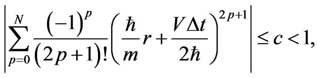 (26)
(26)
where c is a constant. Using a similar argument, we may obtain the same inequality as that in Equation (26) for  Hence, we obtain the following theorem.
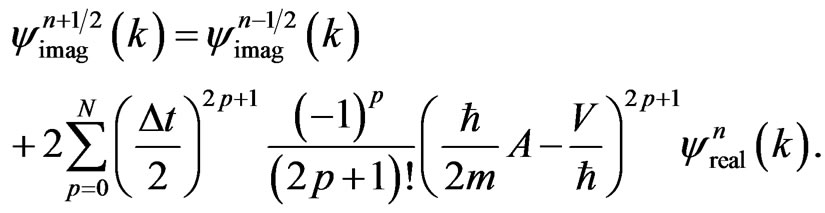
Theorem 1. The generalized FDTD scheme
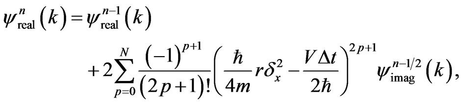 (27a)
(27a)
 (27b)
(27b)
is stable if Equation (26) is satisfied.
It can be seen that when N = 0 the condition in Equation (26) reduces to that in Equation (9). Also, the accuracy of the scheme is 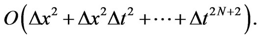
Similarly, for the fourth-order central difference 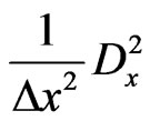 case, we let
 and
and
 and substitute them into Equation (19b). This gives
 (28a)
(28a)
 (28b)
(28b)
Replacing A with  substituting Equation (28)
into Equation (18), and deleting the common factor  we obtain a quadratic equation for
  as follows:
 (29)
(29)
where
Hence, we use a similar argument as before and obtain the following theorem.
Theorem 2. The generalized FDTD scheme
 (30a)
(30a)
 (30b)
(30b)
is stable if the following condition is satisfied
 (31)
(31)
where c is a constant.
The accuracy of the scheme is  It can be seen from the above both schemes that for a larger N, the evaluation for powers of
  or
or  can be very expansive. Therefore, it is our suggestion to choose a smaller N for computation.
4. Absorbing Boundary Condition
When the particle travels and hits the boundary, it will reflect back to the domain under consideration. This will distort the wave packet solution. It is ideal to create an absorbing boundary condition so that the particle will not reflect back. Here, we develop a second-order absorbing boundary condition (ABC) which is obtained from analyzing the group velocity of the wavepacket at the boundaries [15]. To this end, we assume group velocities of the traveling particle to be
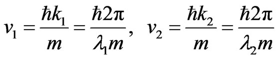 , (32)
where is the wavenumber and
  is the wavelength. By incorporating the dispersion relation
 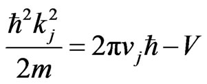 derived from Equation (1), one may see that the wavenumber
 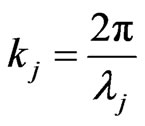 corresponds to
 . Thus, the differential form of the wavenumber can be obtained as
 (33)
(33)
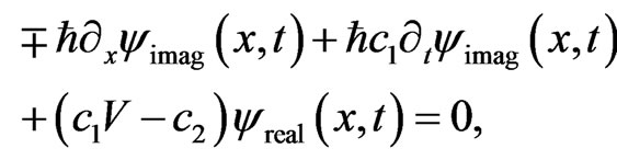
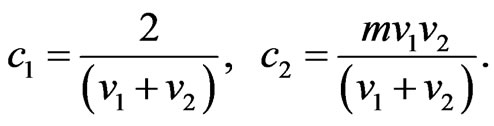
Since a wave maintains various components with different group velocities, we impose a higher-order boundary condition as follows:
 (34)
(34)
It should be pointed out that for a wave traveling towards the left,  and
and  are substituted by
  and
and . It may be seen from Equations (33) and (34) that if
  does not equal
  the two different wave components with group velocities
  and
and  will be absorbed, and on the other hand, if
  is equal to
  the component of the wave with group velocity
  (or
(or ) will be absorbed to the second order.
With Equations (5), (6) and (34), the wavefunctions at the left and right boundaries can be determined as
 (35a)
(35a)
 (35b)
(35b)
where
 (36)
(36)
Here, the upper signs in Equation (35) apply to the left boundary, whereas the lower signs apply to the right. We then use the second-order finite difference schemes to approximate  and
and  at the left
  and right
  boundaries as follows, respectively,
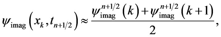 (37a)
(37a)
 (37b)
(37b)
 (37c)
(37c)
and
 , (38a)
 , (38b)
 . (38c)
Upon substituting Equations (37) and (38) into Equation (35), we obtain discrete absorbing boundary conditions as follows:
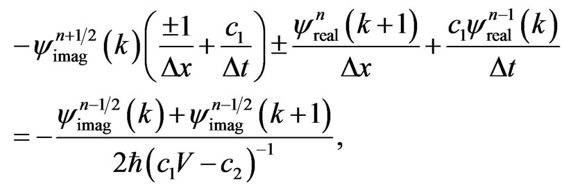 (39a)
(39a)
and
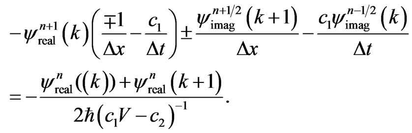 (39b)
(39b)
5. Numerical Examples
To test the stability of the generalized FDTD schemes in Equation (27) and Equation (30) with discrete absorbing boundary conditions, Equation (39), we employed the present schemes and the original FDTD scheme to simulate a particle moving in free space and then hitting an energy potential as tested in [3]. To this end, we initiated a particle at a wavelength of  in a Gaussian envelop of width
  with the following two equations:
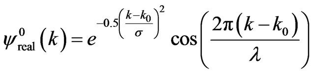 (40a)
(40a)
and
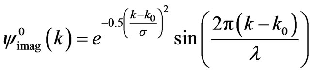 , (40b)
where  is the center of the pulse. We chose a mesh of 1600 spatial grid points and the following values for parameters [3]:
  J×sec,
  kg,
kg,  m,
m,  and
and  m. Furthermore, V was chosen to be 0 in the first 800 grid points and 100 eV in the next 800 grid points.
Two quantities of importance in quantum mechanics are the expected values of the kinetic energy and the potential energy. They are calculated from  and
and  in the simulation as follows,
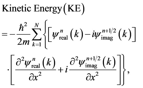 (41b)
(41b)
and
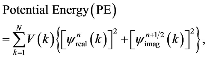 (41b)
(41b)
where 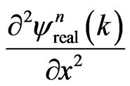 and
and 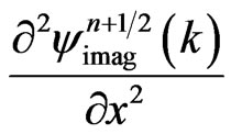 are evaluated using the fourth-order finite difference approximations:
 (42a)
(42a)
and
 (42b)
(42b)
Based on the above formula, the electron moves in free space and then hits an energy potential with a total energy of about 150 eV. The energy is purely kinetic due to the fact that there is no potential energy available before the energy barrier is reached. With an increase in time, the electron will propagate in the positive spatial direction. The waveform begins to spread, but the total kinetic energy remains constant. After the electron strikes the potential barrier, part of the energy will be converted to potential energy. The waveform indicates that there is some probability that the electron is reflected and some probability that it penetrates the potential barrier. However, the total energy should remain constant.
In our computations, we chose N = 2 in Equation (27) and Equation (30), and let
 (43)
(43)
where  is a parameter used in [3]. Using Equation (43), we rewrite the conditions in Equation (26) and Equation (31) for N = 2 as
 (44a)
(44a)
 (44b)
(44b)
Figures 1 and 2 show the simulation of an electron moving in free space and then hitting a potential of 100 eV, which was obtained by using the original FDTD-Q scheme (N = 0) with μ = 0.46875. It can be seen that
when μ = 0.46875 (in which 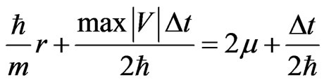
 , the FDTD-Q scheme is stable and indeed the numerical solution does not diverge. Figure 1 shows that when the absorbing boundary condition is not imposed, the wavepacket is distorted at
  On the other hand, Figure 2 shows that the wavepacket disappears at
  when an absorbing boundary condition is imposed. Similar results
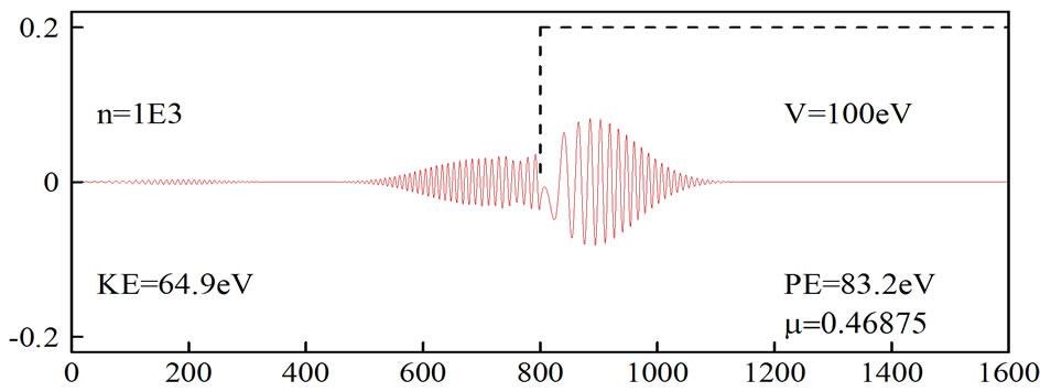
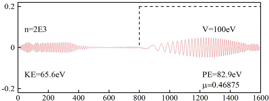
Figure 1. Simulation of an electron moving in free space and then hitting a potential. The original FDTD-Q scheme was employed with µ = 0.46875 and no absorbing boundary condition. Here, the horizontal coordinate is k and the vertical coordinate is ψreal.
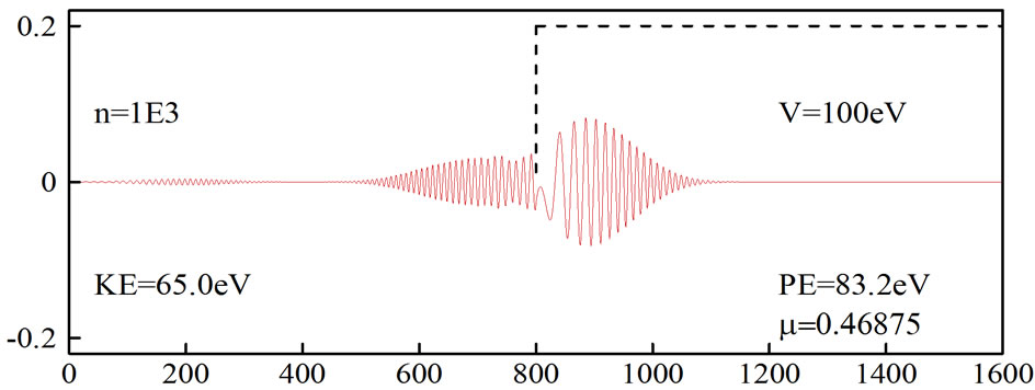
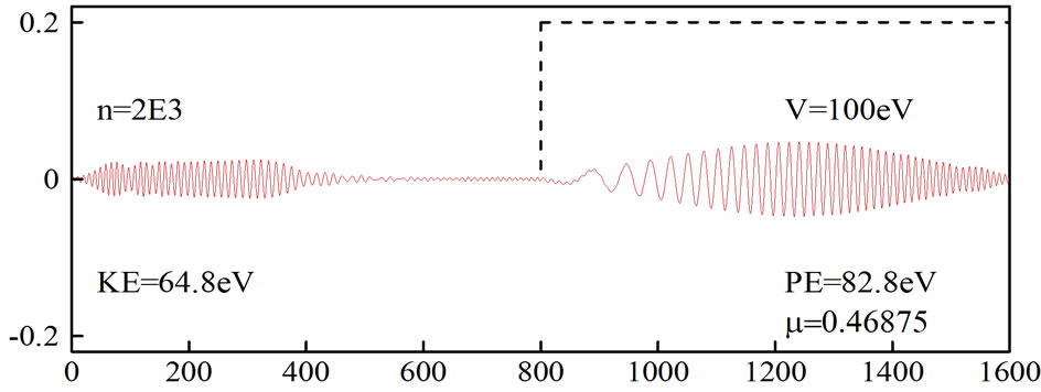
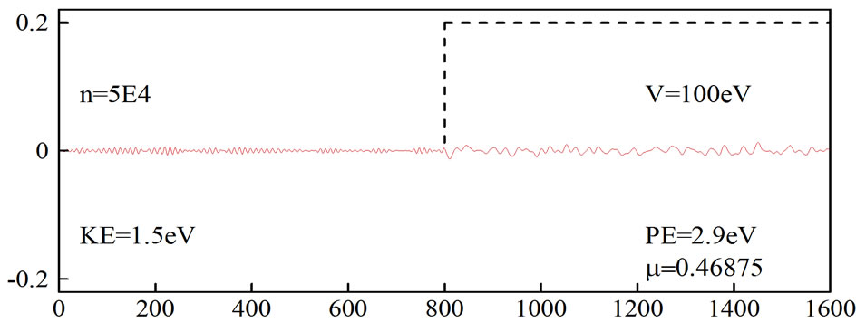
Figure 2. Simulation of an electron moving in free space and then hitting a potential. The original FDTD-Q scheme was employed with µ = 0.46875 and absorbing boundary condition.
are obtained when we used the generalized FDTD scheme (N = 2) with μ = 0.46875.
It is noted that when μ = 0.5 the original FDTD-Q scheme produces a divergent solution, because
 which violates the stability condition. Thus, we employed the generalized FDTD scheme, Equation (27) with N = 2 and Equation (30) with N = 2 for this case. It is noted that when μ = 0.5,
implying the stability condition Equation (26) is satisfied, and
implying the stability condition Equation (31) is satisfied.
Figures 3 and 4 show the simulation of an electron moving in free space and then hitting a potential of 100 eV, which was obtained using the generalized FDTD scheme,

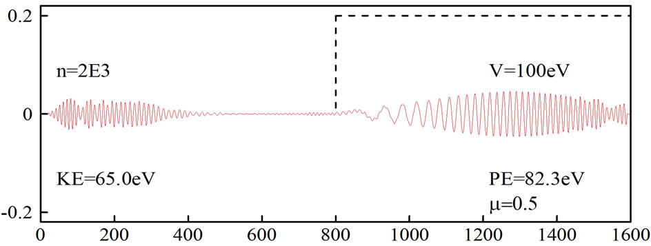
Figure 3. Simulation of an electron moving in free space and then hitting a potential. The second-order FDTD scheme was employed with µ = 0.5 and no absorbing boundary condition.

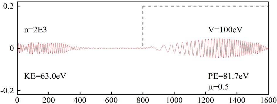
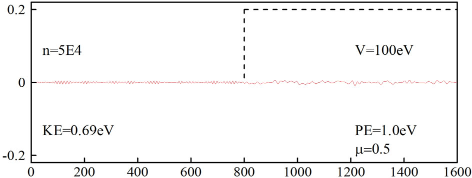
Figure 4. Simulation of an electron moving in free space and then hitting a potential. The second-order FDTD scheme was employed with µ = 0.5 and absorbing boundary condition.
Equation (27) with N = 2 and μ = 0.5. It can be seen from Figure 3 that when the absorbing boundary condition is not imposed, the wavepacket is distorted at  On the other hand, when an absorbing boundary condition is imposed, the wavepacket disappears at
  as shown in Figure 4.
Figures 5 and 6 show the simulation of an electron moving in free space and then hitting a potential of 100 eV, which was obtained using the generalized FDTD scheme, Equation (30) with N = 2 and μ = 0.5. Again, it can be seen from Figure 5 that when the absorbing boundary condition is not imposed, the wavepacket is distorted at  On the other hand, when an absorbing boundary condition is imposed, the wavepacket disappears at
  as shown in Figure 6.
The above numerical example indicates that both generalized FDTD schemes break through the limitation (μ < 0.5) of the original FDTD-Q scheme. It should be pointed out that one may obtain a larger value of μ if N is chosen to be larger in the generalized FDTD scheme.
6. Conclusion
We have developed a generalized FDTD method with absorbing boundary condition for solving the 1D timedependent Schrödinger equation and obtain a more relaxed condition for stability when central difference
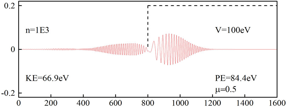
Figure 5. Simulation of an electron moving in free space and then hitting a potential. The fourth-order FDTD scheme was employed with µ = 0.5 and no absorbing boundary condition.

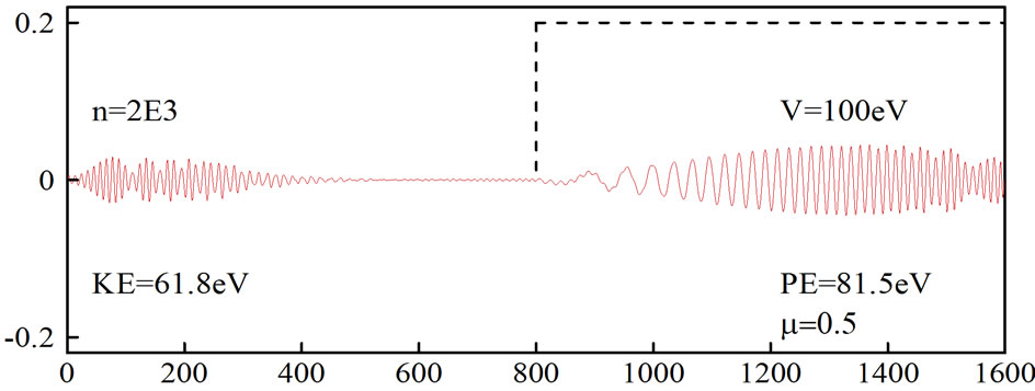
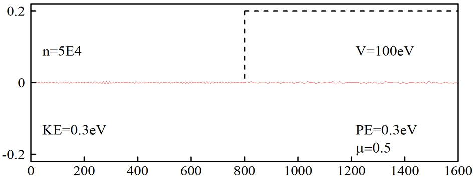
Figure 6. Simulation of an electron moving in free space and then hitting a potential. The fourth-order FDTD scheme was employed with µ = 0.5 and absorbing boundary condition.
approximations are employed for spatial derivatives. Numerical results coincide with those obtained based on the theoretical analysis.
7. Acknowledgements
The research was supported by a grant from the LaSPACE, Louisiana.
REFERENCES
- S. Brandt and H. D. Dahmen, “The Picture Book of Quantum Mechanics,” Springer Verlag, Berlin, 1995. HUdoi:10.1007/978-1-4684-0233-9U
- D. J. Griffiths, “Introduction to Quantum Mechanics. Englewood Cliffs,” Prentice-Hall, Upper Saddle River, 1995.
- D. M. Sullivan, “Electromagnetic Simulation Using the FDTD Method,” IEEE Press, New York, 2000. HUdoi:10.1109/9780470544518U
- P. B. Visscher, “A Fast Explicit Algorithm for the Time Dependent Schrodinger Equation,” Computer Physics, Vol. 5, 1991, pp. 596-598. HUdoi:10.1063/1.168415U
- A. Arnold, M. Ehrhardt and I. Sofronov, “Discrete Transparent Boundary Conditions for the Schrödinger Equation: Fast Calculation, Approximation and Stability,” Communications in Mathematical Science, Vol. 1, 2003, pp. 501- 556.
- A. Askar and A. S. Cakmak, “Explicit Integration Method for the Time-Dependent Schrödinger Equation,” Journal of Chemical Physics, Vol. 68, No. 6, 1978, pp. 2794-2798. HUdoi:10.1063/1.436072U
- W. Bao, S. Jin and P. Markowich, “On Time-Splitting Spectral Approximations for the Schrödinger Equation in the Semiclassical Regime,” Journal of Chemical Physics, Vol. 26, 2005, pp. 487-524.
- N. Carjan, M. Rizea and S. Strottman, “Efficient Numerical Solution of the Time-Dependent Schrödinger Equation for Deep Tunneling,” Romanian Reports in Physics, Vol. 55, 2003, pp. 555-579.
- T. F. Chan, D. Lee and L. Shen, “Stable Explicit Schemes for Equations of the Schrödinger Type,” SIAM Journal on Numerical Analysis, Vol. 23, No. 2, 1986, pp. 274-281. HUdoi:10.1137/0723019U
- H. Chen and B. D. Shizgal, “The Quadrature Discretization Method in the Solution of the Schrödinger Equation,” Journal of Chemical, Vol. 24, 1998, pp. 321-343.
- Z. Chen, J. Zhang and Z. Yu, “Solution of the Time-Dependent Schrödinger Equation with Absorbing Boundary Conditions,” Journal of Semiconductors, Vol. 30, No. 1, 2009, Article ID: 012001. HUdoi:10.1088/1674-4926/30/1/012001U
- W. Dai, “An Unconditionally Stable Three-Level Explicit Difference Scheme for the Schrödinger Equation with A Variable Coefficient,” SIAM Journal on Numerical Analysis, Vol. 29, No. 1, 1992, pp. 174-181. HUdoi:10.1137/0729011U
- W. Dai, G. Li, R. Nassar and S. Su, “On the Stability of the FDTD Method for Solving a Time-Dependent Schrödinger Equation,” Numerical Methods for Partial Differential Equations, Vol. 21, No. 6, 2005, pp. 1140-1154. HUdoi:10.1002/num.20082U
- S. Descomb and M. Thalhammer, “An Exact Local Error Representation of Exponential Operator Splitting Methods for Evolutionary Problems and Applications to Linear Schrödinger Equations in the Semi-Classical Regime,” BIT Numerical Mathematics, Vol. 50, 2010, pp. 729-749.
- T. Fevens and H. Jiang, “Absorbing Boundary Conditions for the Schrödinger Equation,” SIAM Journal on Scientific Computing, Vol. 21, No. 1, 1999, pp. 255-282. HUdoi:10.1137/S1064827594277053U
- F. Fujiwara, “FDTD-Q Analysis of a Mott Insulator Quantum Phase,” Ph.D. Thesis, University of Tokyo, 2007.
- H. Han, J. Jin and X. Wu, “A Finite-Difference Method for the One Dimensional Time Dependent Schrödinger Equation on Unbounded Domain,” Computers and Mathematics with Applications, Vol. 50, No. 8-9, 2005, pp. 1345-1362. HUdoi:10.1016/j.camwa.2005.05.006U
- M. Hochbruuck and C. Lubich, “On Magnus Integrators for Time-Dependent Schrödinger Equations,” SIAM Journal on Numerical Analysis, Vol. 41, 2003, pp. 945-963.
- B. Jazbi and M. Moini, “On the Numerical Solution of One Dimensional Schrödinger Equation with Boundary Conditions Involving Fractional Differential Operators,” IUST International Journal of Engineering Science, Vol. 19, 2008, pp. 21-26.
- Z. Kalogiratou, Th. Monovasilis and T. E. Simos, “Asymptotically Symplectic Integrators of 3rd and 4th Order for the Numerical Solution of the Schrödinger Equation,” Computational Fluid and Solid Mechanics, 2003, pp. 2012-2015.
- K. S. Kunz and R. J. Luebbers, “The Finite Difference Time Domain Method for Electromagnetics,” CRC Press, Roca Raton, 1993.
- J. P. Kuska, “Absorbing Boundary Conditions for the Schrödinger Equation on Finite Intervals,” Physical Review B, Vol. 46, 1992, pp. 5000-5003. HUdoi:10.1103/PhysRevB.46.5000U
- J. Lo and B. D. Shizgal, “Spectral Convergence of the Quadrature Discretization Method in the Solution of the Schrödinger and Fokker-Planck Equations: Comparison with Sinc Methods,” Journal of Chemical Physics, Vol. 125, No. 19, 2006, Article ID: 194108. HUdoi:10.1063/1.2378622U
- P. L. Nash and L.Y. Chen, “Efficient Finite Difference Solutions to the Time-Dependent Schrödinger Equation,” Journal of Chemical Physics, Vol. 130, No. 2, 1997, pp. 266- 268. HUdoi:10.1006/jcph.1996.5589U
- J. M. Sanz-Serna, “Methods for the Numerical Solution of the Schrödinger Equation,” Mathematics of Computation, Vol. 43, 1984, pp. 21-27. HUdoi:10.1090/S0025-5718-1984-0744922-XU
- T. Shibata, “Absorbing Boundary Conditions for FiniteDifference Time-Domain Calculation of the One-Dimensional Schrödinger Equation,” Physical Review B, Vol. 42, 1991, pp. 6760-6763. HUdoi:10.1103/PhysRevB.43.6760U
- A. Soriano, E. A. Navarro, J. A. Porti and V. Such, “Analysis of the Finite Difference Time Domain Technique to Solve the Schrödinger Equation for Quantum Devices,” Journal of Applied Physics, Vol. 95, No. 12, 2004, pp. 8011-8018. HUdoi:10.1063/1.1753661U
- M. Stricklans and D. Yager-Elorriaga, “A Parallel Algorithm for Solving the 3D Schrödinger Equation,” 2010.
- D. M. Sullivan and D. S. Citrin, “Time-Domain Simulation of Two Electrons in A Quantum Dot,” Journal of Applied Physics, Vol. 89, No. 7, 2001, pp. 3841-3846. HUdoi:10.1063/1.1352559U
- D. M. Sullivan and D. S. Citrin, “Time-Domain Simulation of a Universal Quantum Gate,” Journal of Applied Physics, Vol. 96, No. 5, 2002, pp. 3219-3226. HUdoi:10.1063/1.1445277U
- J. Szeftel, “Design of Absorbing Boundary Condition for Schrödinger Equations in Rd,” Journal on Numerical Analysis, Vol. 42, No. 4, 2004, pp. 1527-1551. HUdoi:10.1137/S0036142902418345U
- A. Taflove, Computational Electrodynamics: The FiniteDifference Time-Domain,” Artech House, Boston, 1995.
- L. Wu, “Dufort-Frankel-Type Methods for Linear and Nonlinear Schrödinger Equations,” Journal on Numerical Analysis, Vol. 33, No. 4, 1996, pp. 1526-1533. HUdoi:10.1137/S0036142994270636U
- K. W. Morton and D. F. Mayers, “Numerical Solution of Partial Differential Equations,” Cambridge University Press, London, 1994.