American Journal of Computational Mathematics
Vol.2 No.2(2012), Article ID:20039,7 pages DOI:10.4236/ajcm.2012.22009
Parallel Computing with a Bayesian Item Response Model
1Motorola Mobility, Chicago, USA
2Department of Computer Science, Southern Illinois University, Carbondale, USA
3Department of Educational Psychology & Special Education, Southern Illinois University, Carbondale, USA
Email: *ysheng@siu.edu, rahimi@cs.siu.edu
Received February 4, 2012; revised February 17, 2012; accepted February 25, 2012
Keywords: Gibbs Sampling; High Performance Computing; Message Passing Interface; Two-Parameter IRT Model
ABSTRACT
Item response theory (IRT) is a modern test theory that has been used in various aspects of educational and psychological measurement. The fully Bayesian approach shows promise for estimating IRT models. Given that it is computationally expensive, the procedure is limited in practical applications. It is hence important to seek ways to reduce the execution time. A suitable solution is the use of high performance computing. This study focuses on the fully Bayesian algorithm for a conventional IRT model so that it can be implemented on a high performance parallel machine. Empirical results suggest that this parallel version of the algorithm achieves a considerable speedup and thus reduces the execution time considerably.
1. Introduction
Item response theory (IRT) provides measurement models that describe a probabilistic relationship between correct responses on a set of test items and a latent trait. With many advantages (see [1]), it has been found useful in a wide variety of applications in education and psychology (e.g. [2-4]) as well as in other fields (e.g. [5-10]).
Parameter estimation offers the basis for theoretical advantages of IRT and has been a major concern in the application of IRT models. While the inference of items and persons on the responses is modeled by distinct sets of parameters, simultaneous estimation of these parameters in IRT models results in statistical complexities in the estimation task, which have made estimation procedure a primary focus of psychometric research over decades [11-14]. Recently, because of the availability of high-computing technology, the attention is focused on fully Bayesian estimation procedures, which offer a number of advantages over the traditional method (see e.g. [15,16]). Albert [17] applied Gibbs sampling [18], one of the most efficient Markov Chain Monde Carlo (MCMC [19,20]) algorithms, to the two-parameter normal ogive (2PNO) [21] model. Since a large number of iterations are needed for the Markov chain to reach convergence, the algorithm is computationally intensive and requires considerable amount of execution time, especially with large datasets (see [22]). Hence, achieving a speedup, and thus reducing the execution time, will make it more practical for researchers or practitioners to implement IRT models using Gibbs sampling.
High performance computing (HPC) employs supercomputers and computer clusters to tackle problems with complex computations. HPC utilizes the concept of parallel computing to run programs in parallel and achieve a smaller execution time or communication time, which is affected by the size of the messages being communicated between computers. With parallel computing, many largescale applications and algorithms utilize Message Passing Interface (MPI) standard to achieve better performance. The MPI standard is an application programming interface (API) that abstracts the details of the underlying architecture and network. Some examples of applications that use MPI are crash simulations codes, weather simulation, and computational fluid dynamic codes [23] to name a few.
In view of the above, parallel computing can potentially help reduce time for implementing MCMC with the 2PNO IRT model, and as the size of data and/or chain increases, the benefit of using parallel computing would increase. However, parallel computing is known to excel at tasks that rely on the processing of discrete units of data that are not interdependent. Given the high data dependencies in a single Markov chain for IRT models, such as the dependency of one state of the chain to the previous state, and the dependencies among the data within the same state, the implementation of parallel computing is not straightforward. The purpose of this study is hence to overcome the problem and develop a high performance Gibbs sampling algorithm for the 2PNO IRT model using parallel computing. This paper focuses on all-to-one and one-to all broadcast operations. The aim is to achieve a high speedup while keeping the cost down. The cost of solving a problem on a parallel system is defined as the product of parallel runtime and the number of processing elements used.
The remainder of the paper is organized as follows. Section 2 reviews the 2PNO IRT model and the Gibbs sampling procedure developed by Albert [17]. Section 3 illustrates the approach taken in this study to parallelize the serial algorithm. In Section 4, the performance of the developed parallel algorithm is investigated and further compared with that from serial implementation. Finally, a few summary remarks are given in Section 5.
2. Model and the Gibbs Sampler
The 2PNO IRT model provides a fundamental framework in modeling the person-item interaction by assuming one ability dimension. Suppose a test consists of k multiple-choice items, each measuring a single unified ability, . Let
. Let  represent a matrix of n examinees’ responses to k dichotomous items, so that
  is defined as
 . The probability of person i obtaining correct response for item j can be defined as
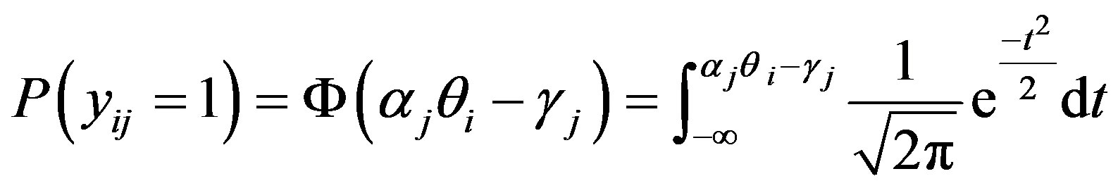 , (1)
, (1)
where  and
and  denote item parameters,
  denotes the continuous person trait parameter, and
  denotes the unit normal cdf.
The Gibbs sampler involves updating three sets of parameters in each iteration, namely, an augmented continuous variable  (which is positive if
  and negative if
 ), the person parameter
 , and the item parameters
 , where
  from their respective full conditional distributions, namely,
 , (2)
, (2)
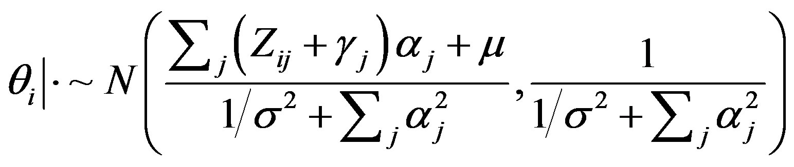 , (3)
, (3)
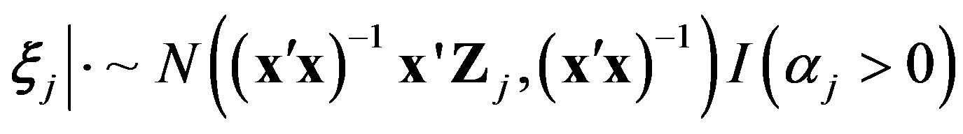 , (4)
, (4)
where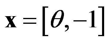 , assuming
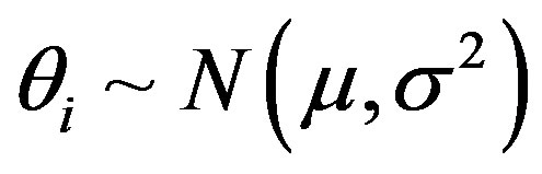 ,
,  and
and 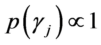 (see [17,22]).
Hence, with starting values  and
and , observations
  can be simulated from the Gibbs sampler by iteratively drawing from their respective full conditional distributions specified in Equations (2), (3) and (4). To go from
  to
to , it takes three transition steps:
1) Draw ;
;
2) Draw ;
;
3) Draw .
.
This iterative procedure produces a sequence of , l = 0, ··· , L. To reduce the effect of the starting values, early iterations in the Markov chain are set as burn-ins to be discarded. Samples from the remaining iterations are then used to summarize the posterior density of item parameters
  and ability parameters
 . The algorithm takes less than 13 minutes for a 2000- by-10 dichotomous (0-1) data matrix and 10,000 total iterations when implemented in Fortran using the Microsoft Powerstation 4.0 compiler and the IMSL Fortran numerical library [22]. For a longer chain with 50,000 iterations, it takes about 60-90 minutes for each execution. With every execution taking more than 12 minutes on a single computer, using this algorithm with large datasets is computational expensive. This further limits the use of IRT models under fully Bayesian framework in various applications.
3. Methodology
The study was performed using the Maxwell Linux cluster, a cluster with 106 processing nodes. Maxwell uses the message passing model via the MPICH MPI framework implementation. One of the 106 nodes acted as the root node, while the rest of the nodes acted as slave nodes. The root node was responsible for generating and partitioning the matrix y, transmitting the submatrices, updating and broadcasting θ, execution time recording, as well as the same duties as the slave nodes.
Each node on the cluster has an Intel Xeon dual CPU quad-core processor clocked at 2.3 GHz, 8 GB of RAM, 90 TB storage, and Linux 64bit operating system. MPICH allows the user to choose how many nodes to use before the execution of a program so that various number of processing nodes may be used in every execution.
3.1. Parallelism with the Gibbs Sampler
When decomposing a problem for parallel computation, the first decomposition method considered is the domain decomposition. In domain decomposition, the data associated with the problem are decomposed and a set of computations is assigned to them [24]. Domain decomposition is a great fit for the 2PNO IRT algorithm since the input and intermediate data can easily be partitioned as illustrated in Figures 1 and 2.
With this approach, the first processing node, P0, receives a sub matrix,  , of size n × g that corresponds to the elements of the y matrix from y0,0 to yn–1, g–1, where
  and P is the number of processing nodes. The second processing node, P1, receives a sub matrix of y,
  , of size n × g that corresponds to the elements of the y matrix from y0, g to yn–1, 2g–1 and so forth. Consequently,
Figure 1. The input y matrix mapped for five processing units.
Figure 2. The Z matrix, and α and γ vectors mapped for five processing units.
each processing node updates the Gibbs samples as in the serial algorithm, but with a smaller input data set. That is, instead of operating on the whole input matrix y, they operate on a part of it of size n × g.
Decompositions of Z, α, and γ are depicted in Figure 2, where we see that each processor is updating a block of Z, α, and γ from Equations (2) and (4), respectively, where j = 1,···, g. For instance, P0 updates a block of Z,  , from Z0,0 to Zn–1, g–1, a block of α,
  , from α0 to αg–1, and a block of γ,
  , from
  to γg–1.
Since θ is of size n × 1 (a column vector), it is not decomposed. However, a problem arises with the update of θ. For simplicity, consider the update of the first element of θ, which requires the updated α, γ, and the first row of Z. Yet, any given processing node has only a part of α, γ, and the first row of Z. The solution is to assign one of the processing nodes (e.g., the root) to update θ and broadcast it to the rest of the units. The naïve approach to update θ would be to have all the units send their part of α, γ and Z to the root so that it has the complete Z, α and γ to update θ from Equation (3) and then broadcast θ to the rest of the nodes. A problem with this approach is that the data communicated are too large, which causes the parallel algorithm to take a longer execution time than the serial algorithm.
A better approach is one that minimizes the communication cost. This can be achieved by having every node to calculate  and
and  and send ψi and τ to the root for it to update q from
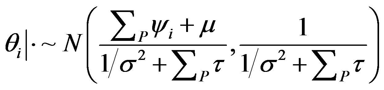 , (5)
, (5)
This way, each processing node is sending a vector of size n + 1 to the root and one message of size n is broadcasted by the root. The total data transferred between all the nodes by this approach is
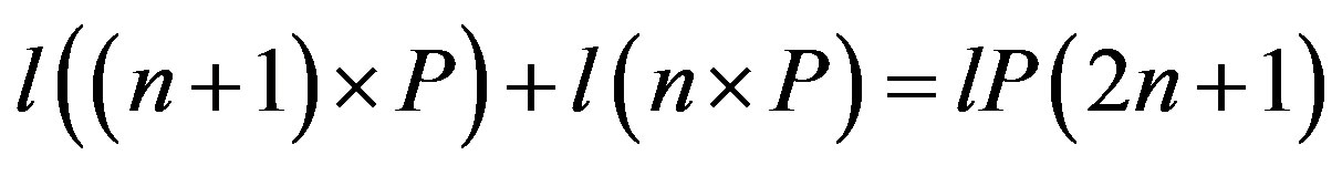 .
.
As a comparison, the total data transferred between all the nodes by the naïve approach is
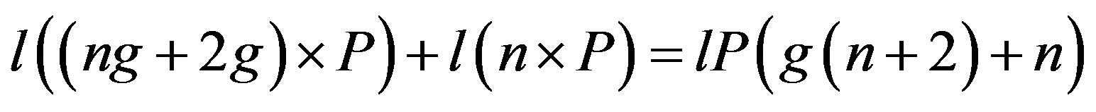 which equals lP(2n + 2) when g = 1, lP(3n + 4) when g = 2, and so forth. When g > 1, the total data transferred using the naïve approach are considerably more than that of the proposed approach (n is usually in the order of thousands).
3.2. Implementation
The proposed algorithm was implemented in ANSI C and MPI with utilization of the GNU Scientific Library (GSL) [25]. To achieve the parallel computation as illustrated in the previous section, the MPI_Gather and MPI_Bcast routines were used for collective communications. See the Appendix for part of the source code of the parallel algorithm in updating the model parameters.
3.3. Performance Analyses
In order to investigate the benefits of the proposed parallel solution against its serial counterpart, four experiments were carried out in which sample size (n), test length (k), and number of iterations (l) varied as below:
Ÿ n =2000, k = 50, l = 10,000Ÿ n =5000, k = 50, l = 10,000Ÿ n =2000, k = 100, l = 10,000Ÿ n =2000, k = 50, l = 20,000.
In all these experiments, one (representing the serial algorithm) to nine processing nodes were used to implement the Gibbs sampler. Their performances were evaluated using four metrics in addition to the execution time. These metrics are the total overhead, relative speedup, relative efficiency, and cost:
Ÿ The total overhead can be calculated as
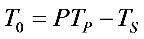 , (6)
, (6)
where P is the number of available processing nodes, TS is the fastest sequential algorithm execution time and TP is the parallel algorithm execution time.
Ÿ Relative speedup is the factor by which execution time is reduced on P processors and it is defined as
 . (7)
. (7)
Ÿ Efficiency describes how well the algorithm manages the computational resources. More specifically, it tells us how much time the processors spend executing important computations [24]. Relative efficiency is defined as
 . (8)
. (8)
Ÿ The definition of cost of solving a problem on a parallel system is the product of parallel runtime and P. Consequently, cost is a quantity that reveals the sum of individual processing node runtime.
4. Results and Discussion
Results from the four experiments are summarized in Figures 3-7. Note that the values plotted represent the average of ten runs. As expected, the execution time decreased as the number of processing nodes increased in all the experimented conditions (see Figure 3).
In terms of efficiency and cost, the algorithm performed better using two to five processing nodes (see Figures 4 and 5). When using up to seven nodes, the communication overhead (see Figure 6) is sufficiently low in order to not affect the overall speedup (see Figure 7). The algorithm had the smallest execution time when
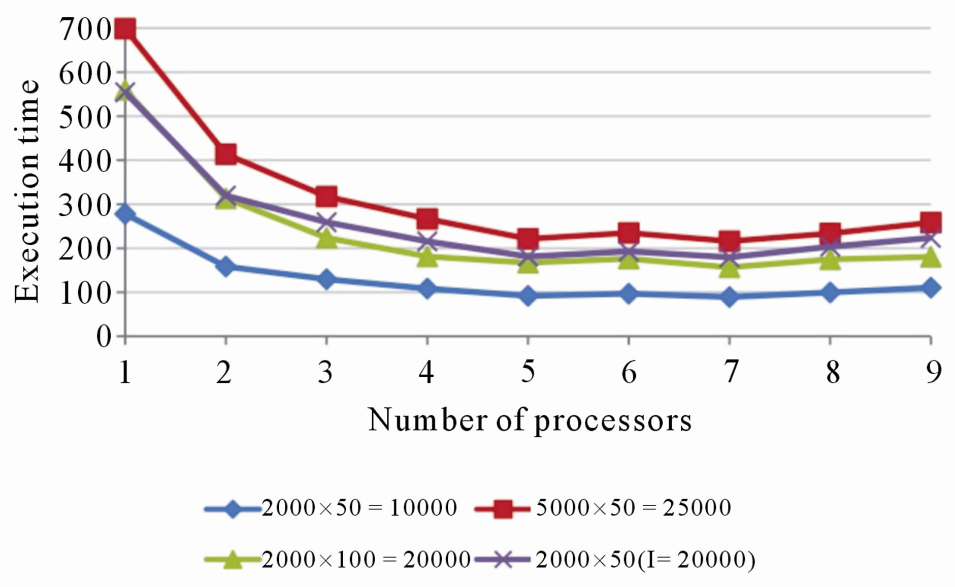
Figure 3. Execution time of the algorithm using one through nine processors in all the experiments.

Figure 4. Relative efficiency of using parallel algorithm over the serial algorithm in all the experiments.
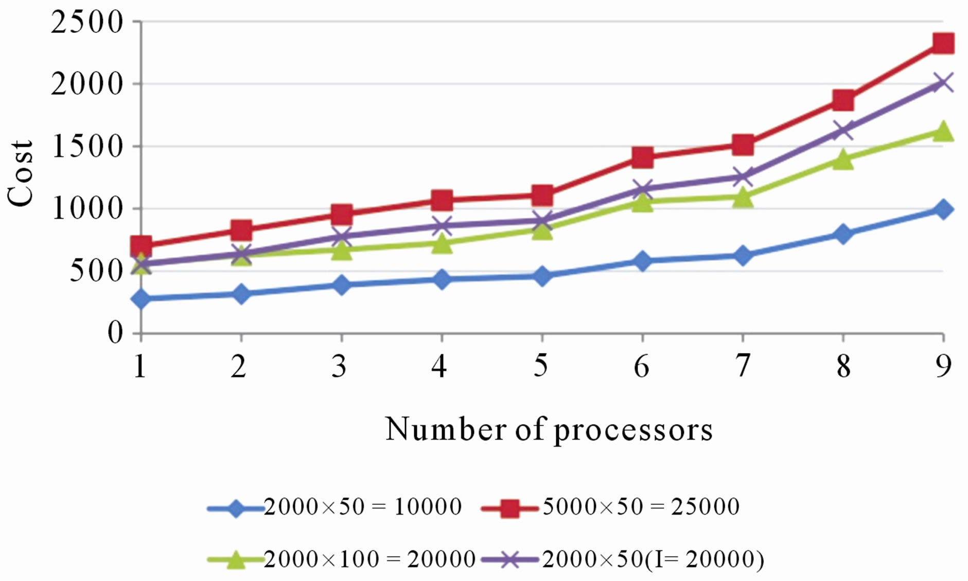
Figure 5. Cost of the algorithm using one through nine processors in all the experiments.
five or seven processing nodes were used (see Figure 3). When nine processing nodes were used, the communication overhead reached the highest, which caused a relatively higher total execution time and lower speedup.
It is noted that the overhead increased as the number of processing nodes increased and it reached the maximum with eight or nine processing nodes. This is because in the parallel algorithm, the overhead of communication is a result of nodes sending ψ and τ to the root and then the root broadcasting θ to the rest of the nodes

Figure 6. Total overhead of using parallel algorithm over the serial algorithm in all the experiments.
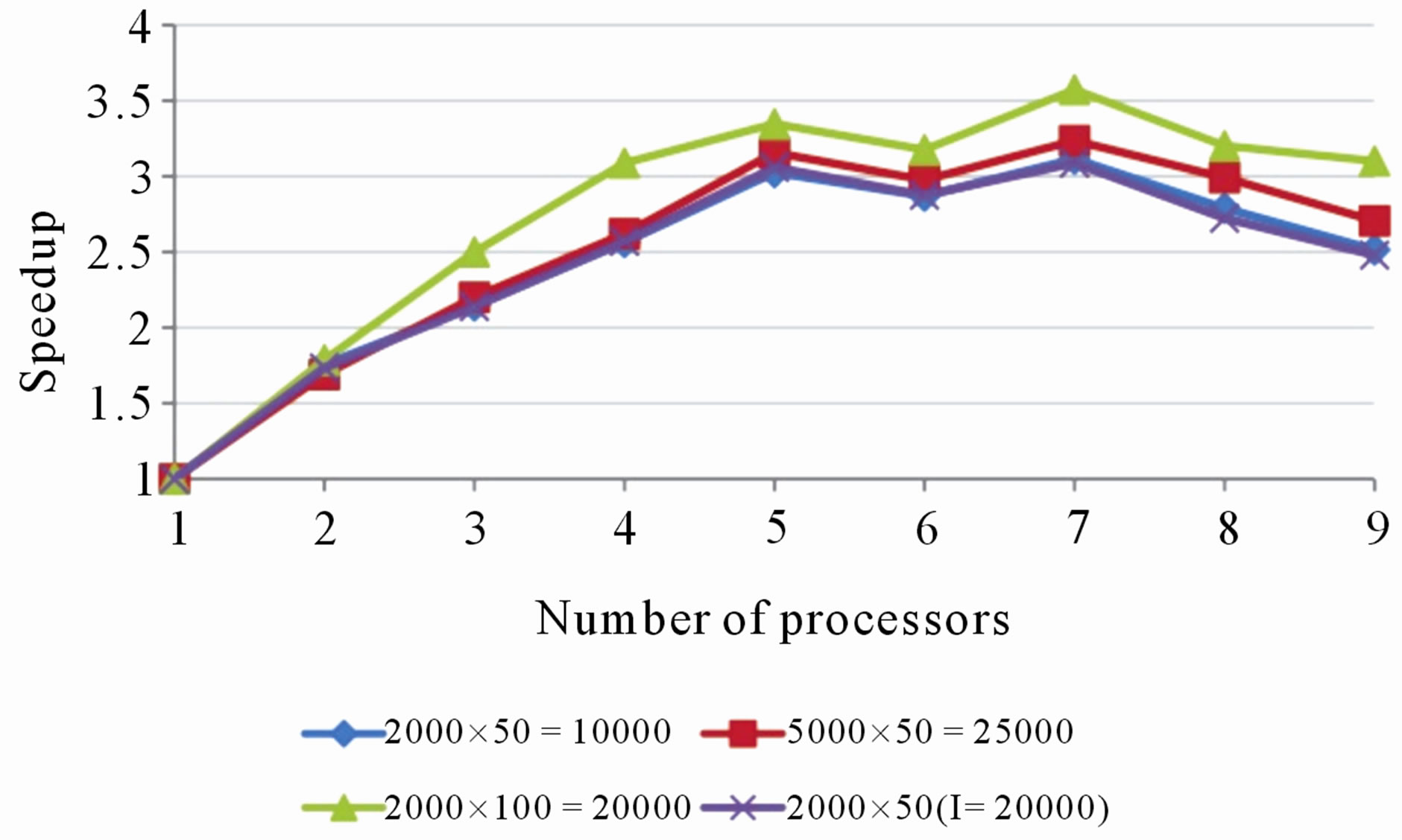
Figure 7. Relative speedup of using parallel algorithm over the serial algorithm in all the experiments.
in every iteration. Note that the total data transferred between all the nodes during execution is lP(2n + 1). The biggest part of idling occurs when the root waits to receive ψ and τ from all the slave nodes and when the slave nodes wait for the root node to calculate θ and broadcast it to them. The communication overhead increases more than the computation speedup when a certain amount of processors are used (ranges from four to seven processors in the experiments performed). As a result, the speedup does not increase with increasing processor count, and consequently, the cost increases dramatically.
Furthermore, a close examination of Figure 7 indicates that the experiments with input matrix sizes 2000 × 50, 5000 × 50, and 2000 × 50 (with number of iterations l = 20,000), follow identical paths. The common input value of these experiments is the number of items, k. The plot for the experiment with input matrix size 2000 × 100 shows that the algorithm maintains a higher speedup compared to the other experiments. Even though the experiment with input matrix size 2000 × 50 has smaller input size, the experiment with input matrix 2000 × 100 maintains a higher speedup over all the processors. The same pattern is observed from Figure 4. In particular, the plot for the experiment with input matrix size 2000 × 100 shows that the algorithm maintains a higher efficiency compared to the other experiments where k = 50. These are because the size of the messages communicated in every iteration from the slave nodes to the root, and from the root to the slave nodes, depends only on n. As k increases, the message size and communication overhead remain unaffected. Because of this, the processors spend more time performing computations and hence the efficiency and speedup increase.
5. Conclusions
This study developed a high performance Gibbs sampling algorithm for the 2PNO IRT model with the purpose of achieving a lower execution time possible using the available hardware (Maxwell cluster). The algorithm was implemented using the ANSI C programming language and the message passing interface. Experiments were performed to evaluate its performance with various dataset sizes or iteration lengths. Results indicated that the parallel algorithm (for the given problem size) performed better, in terms of efficiency and cost, using two to five processing nodes. On the other hand, the algorithm had the smallest execution time when nine processing nodes were used.
The design of a parallel 2PNO IRT model has proved to be justifiable. Given the high data dependencies for such problems, the solution initially appeared to be non-trivial. By using domain decomposition, we managed to avoid communication for the state dependencies. Nevertheless, communication in every iteration of the Markov chain cannot be avoided because of the data dependencies within the state. By modifying the serial algorithm, the size of the data communicated in every iteration was managed to be reduced to make a speedup possible.
This study achieved parallelization through a columnwise decomposition and the use of all-to-one and oneto-all broadcast schemes. Further studies can be undertaken to increase the speedup and the efficiency, and minimize the cost and the total overhead. For example, the data may be decomposed differently or an all-to-all broadcast scheme may be adopted in order to achieve smaller communication overhead.
REFERENCES
- R. Hambleton, H. Swaminathan and H. J. Rogers, “Fundamentals of Item Response Theory,” Sage Publications, Thousand Oaks, 1991.
- M. J. Kolen and R. L. Brennan, “Test Equating: Methods and Practices,” Springer-Verlag, New York, 1995.
- S. E. Embretson and S. P. Reise, “Item Response Theory for Psychologist,” Lawrence Erlbaum Associates Inc., Mahwah, 2000.
- H. Wainer, N. Dorans, D. Eignor, R. Flaugher, B. Green, R. Mislevy, L. Steinberg and D. Thissen, “Computerized Adaptive Testing: A Primer,” Lawrence Erlbaum Associates Inc., Mahwah, 2000.
- J. Bafumi, A. Gelman, D. K. Park and N. Kaplan, “Practical Issues in Implementing and Understanding Bayesian Ideal Point Estimation,” Political Analysis Advance Access, Vol. 13, No. 2, 2005, pp. 171-187. doi:10.1093/pan/mpi010
- N. Bezruckzo, “Rasch Measurement in Health Sciences,” JAM Press, Maple Grove, 2005.
- C. H. Chang and B. B. Reeve, “Item Response Theory and Its Applications to Patient-Reported Outcomes Measurement,” Evaluation & the Health Professions, Vol. 28, No. 3, 2005, pp. 264-282. doi:10.1177/0163278705278275
- U. Feske, L. Kirisci, R. E. Tarter and P. A. Plkonis, “An Application of Item Response Theory to the DSM-III-R Criteria for Borderline Personality Disorder,” Journal of Personality Disorders, Vol. 21, No. 4, 2007, pp. 418-433. doi:10.1521/pedi.2007.21.4.418
- G. W. Imbens, “The Role of the Propensity Score in Estimating Dose-Response Functions,” Biometrika, Vol. 87, No. 3, 2000, pp. 706-710. doi:10.1093/biomet/87.3.706
- S. Sinharay and H. S. Stern, “On the Sensitivity of Bayes Factors to the Prior Distribution,” The American Statistician, Vol. 56, No. 3, 2002, pp. 196-201. doi:10.1198/000313002137
- A. Birnbaum, “Statistical Theory for Logistic Mental Test Models with a Prior Distribution of Ability,” Journal of Mathematical Psychology, Vol. 6, No. 2, 1969, pp. 258- 276. doi:10.1016/0022-2496(69)90005-4
- F. B. Baker and S. H. Kim, “Item Response Theory: Parameter Estimation Techniques,” 2nd edition, Dekker, New York, 2004.
- R. D. Bock and M. Aitkin, “Marginal Maximum Likelihood Estimation of Item Parameters: Application of an EM Algorithm,” Psychometrika, Vol. 46, No. 4, 1981, pp. 443-459. doi:10.1007/BF02293801
- I. W. Molenaar, “Estimation of Item Parameters,” In: G. H. Fischer and I. W. Molenaar, Eds., Rasch Models: Foundations, Recent Developments, and Applications, SpringerVerlag, New York, 1995, pp. 39-51.
- R. K. Tsutakawa and J. C. Johnson, “The Effect of Uncertainty of Item Parameter Estimation on Ability Estimates,” Psychometrika, Vol. 55, No. 2, 1990, pp. 371-390. doi:10.1007/BF02295293
- R. K. Tsutakawa and M. J. Soltys, “Approximation for Bayesian Ability Estimation,” Journal of Educational Statistics, Vol. 13, No. 2, 1988, pp. 117-130. doi:10.2307/1164749
- J. H. Albert, “Bayesian Estimation of Normal Ogive Item Response Curves Using Gibbs Sampling,” Journal of Educational Statistics, Vol. 17, No. 3, 1992, pp. 251-269. doi:10.2307/1165149
- S. Geman and D. Geman, “Stochastic Relaxation, Gibbs Distributions, and the Bayesian Restoration of Images,” IEEE Transactions on Pattern Analysis and Machine Intelligence, Vol. 6, No. 6, 1984, pp. 721-741. doi:10.1109/TPAMI.1984.4767596
- A. F. M. Smith and G. O. Roberts, “Bayesian Computation via the Gibbs Sampler and Related Markov Chain Monte Carlo Methods,” Journal of the Royal Statistical Society, Series B, Vol. 55, No. 1, 1993, pp. 3-24.
- L. Tierney, “Markov Chains for Exploring Posterior Distributions (with discussion),” Annals of Statistics, Vol. 22, No. 4, 1994, 1701-1762. doi:10.1214/aos/1176325750
- F. M. Lord and M. R. Novick, “Statistical Theories of Mental Test Scores,” Addison-Wesley, Boston, 1968.
- Y. Sheng and T. C. Headrick, “An Algorithm for Implementing Gibbs Sampling for 2PNO IRT Models,” Journal of Modern Applied Statistical Methods, Vol. 6, No. 1, 2007, pp. 341-349.
- R. Noronha and K. P. Dhabaleswar, “Performance Evaluation of MM5 on Clusters with Modern Interconnects: Scalability and Impact,” Euro-Par 2005 Parallel Processing, 2005, Vol. 3648, pp. 134-145. doi:10.1007/11549468_18
- I. Foster, “Designing and Building Parallel Programs: Concepts and Tools for Parallel Software Engineering,” Addison-Wesley, Boston, 1995.
- M. Galassi, J. Davies, J. Theiler, B. Gough, G. Jungman M. Booth, et al., “GNU Scientific Library Reference Manual,” 2009. http://www.gnu.org/software/gsl
Appendix
The pseudo code for updating the values of Z, ψ, τ, θ, α, and γ is shown below. First of all, Z is updated through the function update_Z. Then, update_PSI_TAU is called to update ψ and τ and MPI_Gather is called to send ψ and τ to the root. The root receives ψ and τ and calls update_TH to update θ and afterwards broadcasts θ by calling MPI_Bcast. Finally, α and γ are updated from a function call to update_A_G. In order to reduce communication overhead, ψ and τ are sent in the same message. To achieve that, an array of size n +1 is set up, where the first n entries consist of the elements of ψ and entry n +1 consists of τ (the name of this array in the code is PSI_TAU_array).
// Start iteration:
for (m = 0; m < l; m++){
count++;
update_Z(Z, y, TH, A, G, r);
update_PSI_TAU(PSI_TAU_array, Z, A, G);
MPI_Gather (PSI_TAU_array, n+1MPI_DOUBLE, PSI_TAU_rec, n+1, MPI_DOUBLEROOT, MPI_COMM_WORLD);
if (rank == ROOT){ double TAU_array[size]; int ind = 0;
// Retrieve PSI and TAU from PSI_TAU_rec:
for (j = 0; j < size; j++){
for (i = 0; i < n+1; i++){
if (i < n)
gsl_matrix_set(PSI_matrix, i, jPSI_TAU_rec[ind++]);
else TAU_array[j] = PSI_TAU_rec[ind++];
}
}
update_TH (TH, THV, TAU_array, PSI_matrix, count, r);
// Transfer TH data into a buffer so that it can be broadcasted:
for (i = 0; i < n; i++){
TH_array[i] = gsl_vector_get(TH, i);
}
}
MPI_Bcast (TH_array, n, MPI_DOUBLE, ROOT, MPI_COMM_WORLD);
// Transfer TH received to a vector structure:
for (i = 0; i < n; i++){
gsl_vector_set (TH, i, TH_array[i]);
}
update_A_G(A, G, AV, GV, Z, TH, unif, count, r, p);
} // end iteration
NOTES
*Corresponding author.