American Journal of Computational Mathematics
Vol.2 No.1(2012), Article ID:17951,11 pages DOI:10.4236/ajcm.2012.21001
Solution Building for Arbitrary System of Linear Inequalities in an Explicit Form
Energy Research Institute, Russian Academy of Sciences, Moscow, Russia
Email: *macro@eriras.ru
Received November 25, 2011; revised January 16, 2012; accepted January 28, 2012
Keywords: Linear Inequalities; Convolution; Variable Elimination; Orthogonal Projection Method; Fourier Algorithm; Chernikov Rules; Dependent Inequalities; Redundant Inequalities; Almost Dependent Inequalities; Matrix Cleanup; Coarsening
ABSTRACT
The known Fourier-Chernikov algorithm of linear inequality system convolution is complemented with an original procedure of all dependent (redundant) inequalities deletion. The concept of “almost dependent” inequalities is defined and an algorithm for further reducing the system by deletion of these is considered. The concluding algorithm makes it possible to hold actual-time convolution of a general inequality system containing up to 50 variables with the rigorous method of dependent inequalities deletion and up to 100 variables with the approximate method of one. The main application of such an approach consists in solving linear inequality system in an explicit form. These results are illustrated with a series of computer experiments.
1. Introduction
Polyhedron orthogonal projection (POP) was devised by Fourier [1] as early as in the 20s of the XIX century. Some properties of an arbitrary convex set orthogonal projection are considered by Shapot [2]. However, the closed algorithm of generating orthogonal projections to any subspaces is known only for linear polyhedral sets. For a long time the POP didn’t find obvious practical use as with every elimination of variables it initiated a large number of dependent (redundant) inequalities. It resulted in a rapid increase in their total number and as a rule didn’t make it possible to solve the problem within an acceptable timeframe. In the middle of the XX-th century Chernikov [3] devised methods of dependent inequality determination, making substantial progress towards resolving this problem. With their help it became possible to increase the dimension of the problem, solved with POP within acceptable time, from 5 - 8 to 8 - 15, however, a further increase of dimensions resulted in the former problems of expansion. Methods of dependent inequalities in large linear systems determination began to develop in the 80s (ref., for example, Bushenkov and Lotov [4], Lotov [5], Eremin and Makhnev [6]). A new constructive approach to the implementation of the Fourier-Chernikov algorithm (FCA), which makes it possible to control inequality number expansion during the process of variable elimination, was devised by Shapot and Lukatskii [7]. From this point on we shall refer it to as the constructive algorithm of convolution—CAC.
Here we give a preliminary formulation of the main algorithm. Let the  system be given, enclosing k of linear equations and m of linear inequalities, defining non-empty set in real space
 . Let us suppose that the
  investigation aim is to find its nonbasic variable population and to write each of them in an explicit form. Such a notation can be represented in two ways: 1) in the form of this variable equality to a number or to a linear function of numerically defined variables; 2) in the form of value bounds restricted by either numbers or by linear functions, which depend on previously numerically defined variables. Previously defined variable numerical values” should be considered only within the framework of a procedure containing the following two stages:
Ÿ Elimination of all equations from  by means of “Step of Jordan Elimination” (JE) series. Then
  of variables will be assumed to be set equal to the linear functions, which depend on the rest
  variables, where
  of the equation subsystem (
 , if all equations are mutually independent). These variables will gain numerical values after solution of the remaining system of inequalities
  to
to . Let us suppose that every inequality defines non-negativity of the corresponding basic variable.
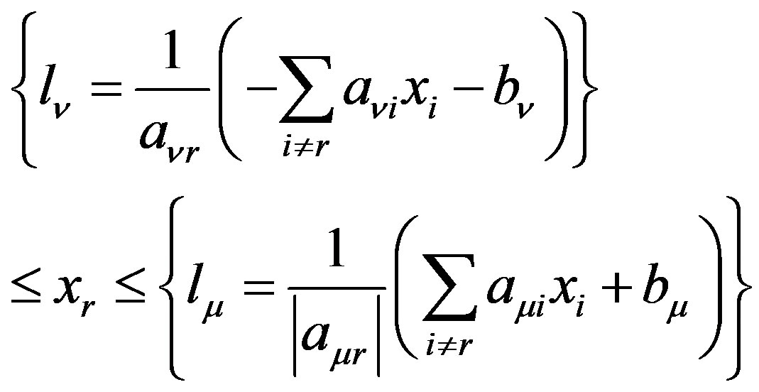
Ÿ  “inequality system solution” is generated by an investigator in the form of an arbitrary sequence of p variables, in which the first variable has one or two numerical boundaries and each of the consequent variables is limited by linear functions, which depend on previously considered variables. Such a pyramidal (
 ) representation of inequality system
  is similar to limit defining in multiple integrals. With such a representation it is quite convenient to select a working point in
 , being guided by some conceptual criteria.
Let us consider an algorithm of  sequence generation. Let us compare
  inequality system with the matrix
 , which defines p-dimensional convex polyhedron. Let us decrease its dimension to
 , i.e. let us pass to the matrix
 , eliminating an arbitrary variable
  from the coordinate set. This can be done in two ways: either by assigning a numerical value to
 , i.e. by making
 , section or by constructing the union of all sections along
 , i.e. the
  orthogonal projection on subspace not containing
 . We will use the second way of eliminating variables. Let us generate
  matrix sequence with
  polyhedra decreasing dimensions. Precisely this sequence will make it possible to easily generate
 . Really the
  matrix contains only two columns, the first with the coefficients
  corresponds to
  variable and the other one with the coefficients
 —to free members.
Denote by 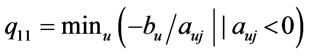 and
and
 .
.
Then it is not too difficult to see that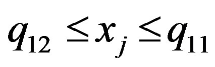 , where
  and
and  are numbers. In the same way it is possible to represent the bounds for
  variable using the
  matrix with the
  and
and  variables,
  , where
  and
and  are linear functions, which depend on
 . If you select
  “attractive” value within the specified range, the
  acceptable range will be a numerical one. This method of boundary function
  matrix construction and the selection of variable “attractive” values can be prolonged to the
  parent matrix. From this point on we shall refer the considered approach to as POP.
Fourier algorithm is described in Section 2. Different methods of redundant inequality cleanup are considered and a formal description of POP is given in Section 3. The stability and complexity of POP algorithms are estimated in Section 4. The results of numerical experiments are discussed in Section 5.
2. Orthogonal Projection Fourier Algorithm
Let  be a real n-dimensional space. The set
is referred to as the  set projection on the
  subspace.
Let us consider the  non-empty bounded set, defined by the linear system of inequalities
 .
.
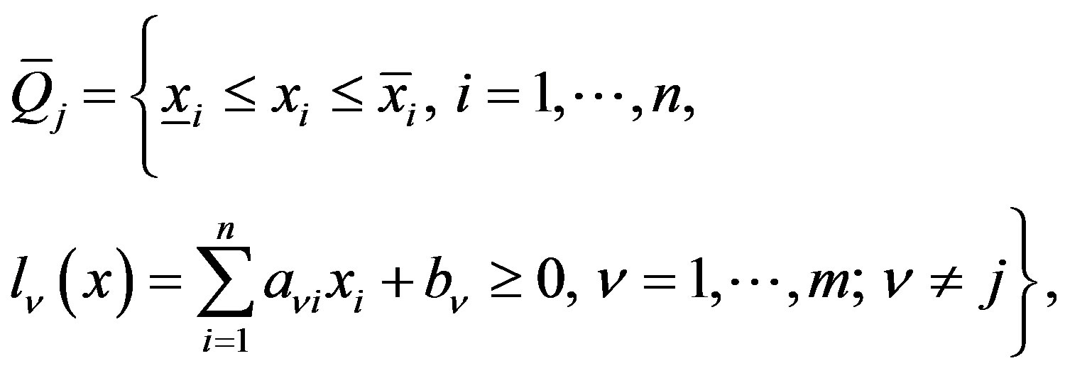
Suppose we want to build , where
  doesn’t depend on an
  variable. According to the algorithm of linear inequality systems free convolution devised by Fourier [1] let us divide J index set into three groups:
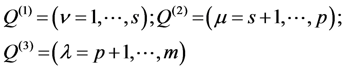
so, that for them .
.
Solving each of two first groups of inequalities with respect to  we obtain
 (1)
(1)
Eliminating  from these relations, i.e. combining each inequality of the first group with each inequality of the second group we obtain
 , generated by
  inequalities, which have the form
 (2)
(2)
and  inequalities of the third group.
As a matter of fact, 
and then 
 .
.
On the other hand, if  doesn’t comply with the
  -th inequality of (2), then any
 , complying with the
  inequality of (1), contradicts the
  -th inequality and vice versa.
If the first or the second group of inequalities is empty, i.e. , then for any
 , complying with inequalities of the third group,
  and for any
  Therefore, in this case
 .
.
With the help of the considered algorithm it is possible to eliminate any subset of variables and to construct the  orthogonal projection, where
  Since all computations are performed in the form of a matrix notation, the
  set is defined by the matrix, which we shall denote as
 . Then the
 , projection generated as a result of eliminating k variables, is defined by the
  matrix. If
 , then the
  contains only
  column and the column of constant term. The (1) formula, which corresponds to it, has the form:
  where
where 
 Such a notation makes it possible to select any value of
  variable of the
  projection on the
  axis, i.e. a permissible value. The same situation will occur, if in the
  matrix you multiple the
  column by
 . And in general, during “the descent from the sequence of
  matrices” after selection of the
  variables arbitrary permissible values and multiplying the
  matrix corresponding columns by them we shall obtain the acceptable range for the
 .variable value selection. Therefore, it is possible to say, that the
  matrix sequence allows us to obtain in explicit form the solution of the inequality system defined by
 .
.
The considered Fourier algorithm, in spite of its seeming simplicity, is usable only for the simplest systems of inequalities. The necessity of all  -th pairs combining while eliminating each variable causes a rapid expansion of inequality number with elimination of variables. In particular, if after
  variable elimination a system of
  inequalities is obtained, then after k-th variable elimination we shall obtain
  . The
. The  lower boundary is implemented in the case if
  and
and , or
, or , and the upper boundary if
  and
and . Here a large percentage consists of generated inequalities are dependent. So, if
 , then the accessible upper bound for
  is
is  of inequalities.
Thus, intensive expansion of inequality number with elimination of variables is the main obstacle for POP use in problems of practical importance. To overcome this obstacle it is first of all necessary to have effective algorithms for determination of dependent inequalities generated while using the Fourier algorithm. From this point on we shall refer to them as “matrix cleanup” algorithms.
3. Methods of Eliminating Dependent Inequalities
3.1. Fourier-Chernikov Algorithm (FCA)
Motzkin et al. [8] and Chernikov [3] offered a serious improvement to the Fourier algorithm related to the abandonment of generating some dependent inequalities. By endowing each inequality of parent system with a primary subscript (number) and by joining (disjuncting) the subscripts while combining inequalities in pairs Chernikov complemented the Fourier algorithm with the following two rules:
(ChR1) With eliminating the  -th in succession inequality only those inequalities which generate the subscript containing not more than
  of primary subscripts are to be combined (Chernikov’s first rule);
(ChR2) The pairs containing some other inequality total subscript shouldn’t be combined in pairs (Chernikov’s second rule).
In FCA (ChR1) is verified during the process of Fourier inequalities combining and the (ChR2) is verified after all combinations not contradicting (ChR1) have been generated. With the help of Chernikov’s rules all dependent inequalities are determined in the total polyhedra assembly, i.e. for all systems of homogeneous inequalities. However, for the inequalities with fixed constant terms these rules do not by any means determine all dependent inequalities.
The validity of this statement is readily illustrated by simple numerical examples. To generate them and to conduct consequent computational experiments we used general linear programming (LP) generator of inequality system:
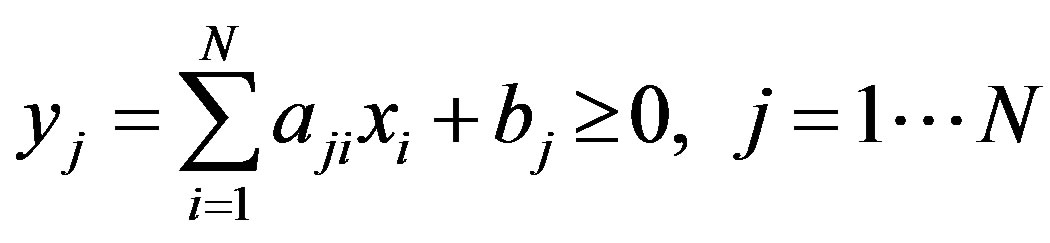 where
where
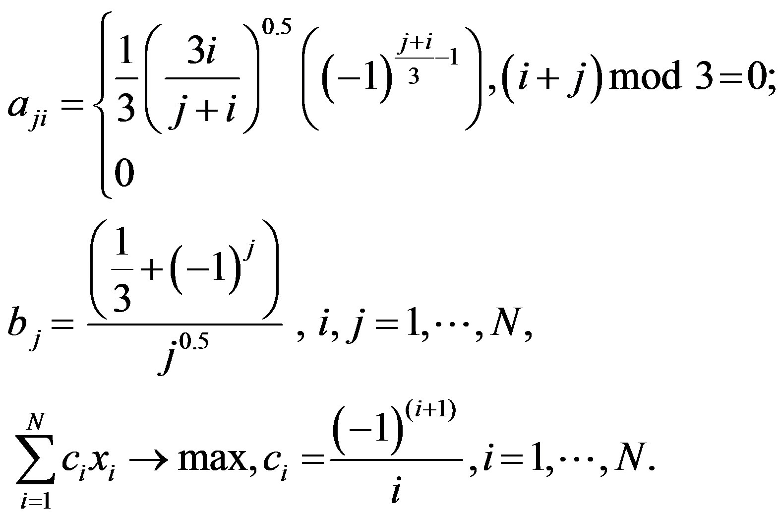 (3)
(3)
The bounds of nonbasic variable are:
 .
.
In the first example for the case where  and using the Fourier algorithm without applying Chernikov’s rules 587115 inequalities were generated with the elimination of the 7-th variable. In the case where N = 8 the use of the Fourier algorithm led to the memory overflow. In the second example where
 , application of Chernikov’s rules, but without determination of all redundant inequalities, generated the results given in Table 1. But if you use the algorithm of dependent inequality complete cleanup in this example, convolution results will appear to be quite different. They are given in Table 2.
Thus, the prospects for practical use of convolution
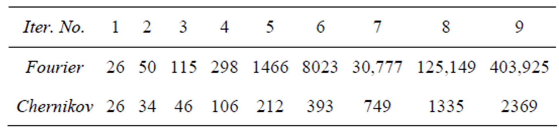
Table 1. No determination of all redundant inequalities.

Table 2. With determination of all redundant inequalities.
algorithms substantially depend on the possibility of determination of dependent inequalities generated in the framework of FCA. It should be pointed out, that Chernikov [3] also considered the method of all redundant inequalities with fixed constant terms complete cleanup. It is based on a computation of cone generator fundamental system associated with the system of linear inequalities. According to Preparata and Shamos [9], Shevchenko and Gruzdev [10] the corresponding algorithm has an operation number polynomial estimator on linear inequality system cardinality with a fixed dimension. In particular, if  is the inequality number (cardinality), n is the variable number (dimension), then the operation number in this algorithm has the estimate
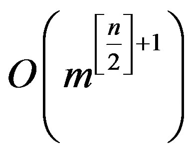 . As the number of inequalities can increase rapidly during the convolution process, such algorithm use does not seem to be of practical importance.
3.2. A Formalized Description of POP
Step 0. Clear the counter of variable eliminations .
.
Read an initial matrix  of the linear inequality system, where
 —the number of variables.
Endow each linear inequality  a primary subscript
 .
.
Step 1. Choose a column , which has
  positive and
  negative elements, and multiplication
  being minimal. If such a column is absent, then procedure is complete, otherwise
 .
.
Note, that under parallelepiped restrictions on all variables a premature end is possible only for an incompatible system, as otherwise there would be a non bounded variable, in the contrary system.
Step 2. Exclude the variable  by (1), (2) formula from the inequality system. As each new inequality is generated, let us form its subscript
  by uniting the subscripts of the corresponding pair. We do not include the inequalities being redundant with the 1-st Chernikov rule, i.e. number of primary indexes (ChR1)
 don’t include in the system.
Step 3. Carry out a control of subscript pairs on (ChR2) ( ), then delete the inequality with subscript
  from the system as a redundant one.
Step 4. Carry out after the full cleanup in the inequality system.
Step 5. Save  matrix
  -th iteration of inequality system and the number
  of excluding variable. If
 , then return to Step 1, otherwise the end.
3.3. The Algorithm of Building of an Inequality System Solutions in Explicit Form
Here we give a formal description of the algorithm in 1.
This procedure means that all  steps of variable elimination have been implemented. Then the matrix
  contains the single variable with number
  and the matrix
  contains
  variables with numbers
 .
.  is the initial matrix of linear problem with
  variables.
For  do Step
 . If
. If , then go to 2, otherwise:
1. In the matrix  we fix the values of variables, which were changed in the preceding steps

as a result the matrix  contains the single variable
 .
.
2. Using the matrix , the solution of an inequality system with this single variable is formed as the range of its acceptable values:
  . We choose a desired value
  from this range. If
 , then
  and return to 1, otherwise the end.
3.4. Constructive Approach to Determination of Dependent Inequalities in Polyhedral Sets
The problem of dependent inequalities determination is rather relevant for various applications. It was considered by many authors both in the context of projections method Bushenkov and Lotov [4], Lotov [5], Eremin and Makhnev [6] and independently Efremov, Kamenev and Lotov [11], Golikov and Evtushenko [12], Gutman and Ioslovich [13], Paulraj and Sumathi [14]. Before we developed and programmatically implemented several approaches to the determination of dependent inequalities in linear systems Shapot and Lukatskii [7,15]. We describe and substantiate the algorithm of Shapot and Lukatskii [7] further in this text.
In spite of the fact that the problem of dependent inequalities determination after FCA algorithm iteration is considered, the devised algorithm is of a general nature and is not associated with the orthogonal projection specific procedure. To ensure investigated polyhedron boundedness we require that the upper and lower boundaries are defined for all free variables. These boundaries shall define the survey coverage of models in the form of a rectangular parallelepiped, of interest for the investigator. However, in the case when any of parallelepiped restrictions appears to be dependent it should be eliminated from the corresponding matrix like any other dependent inequality. Here we remind the dependent inequality concept.
Definition 3.1. The inequality  is dependent (redundant) on a set
 , if it is satisfied in each point of this set and is incompatible with
 , if it is satisfied in no point
The analysis of  inequality dependence or incompatibility conditions with respect to the
  set can be founded on any of the following equivalent and obvious criteria.
(Crit1) In order for the  inequality could be:
a) dependent on , or b) incompatible with
 It is necessary and sufficient to meet the conditions:
a)  r b)
r b) .
.
(Crit2) The  inequality is dependent on
  if and only if It is representable as
 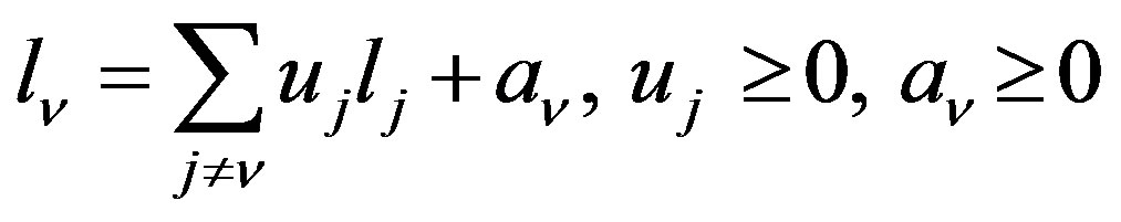 Chernikov [3].
(Crit3) a) Elimination of any independent inequality from the system of inequalities causes region of feasibility expansion, i.e.  and
and ;
;
b) Elimination of any dependent inequality from the system of inequalities doesn’t cause region of feasibility expansion, i.e. .
.
In the general case, when the  inequality dependence on the
set is investigated it is sufficient to use (Crit1) and to solve the corresponding problem of linear programming (LP). However, we are interested in the complete cleanup of matrix in the framework of orthogonal projecting procedure (OPP), when inequalities number rapid expansion is possible with variables elimination. Suppose, that at the OPP next step after FCA implementation the generated system of m inequalities can contain noticeable amounts of dependent inequalities. In this situation the approach based on (Crit1) direct use for m inequalities testing assumes LP  problems solving. It is obvious that such an approach is not attractive. Let us consider a fundamentally different way of slump in amount of corresponding computation while verifying inequalities independence.
Suppose that a basic solution is found for the linear inequality system defining  -dimensional compact polyhedral set
 (4)
(4)
obtained after the OPP next step and containing no pairwise equivalent inequalities. As a reminder, some solution of (4) is referred to as a basic one if it satisfies all constraints and transforms at least n inequalities into equalities. Relying on the conditions considered below we can verify dependence of all inequalities corresponding to the basic solution matrix (BSM). We shall first make some terms more precise.
By using variable shift we may reduce our problem to the case . We also transform
  to the form
  and add it to the constrain set
 . Below we shall refer to the
  variables in the formula (4) as nonbasic (free) ones and the
  variables—as basic (constrained) ones. Moreover, in respect of any simplex-matrix we shall speak of column and row variables. Any of these variables is associated with its non-negativity condition. Therefore, each inequality corresponds to one of the variables.
From this point onwards we shall refer to the difference between the dependence in respect of the  set and the
  dependent inequality:
Definition 3.2. The  is the first kind, if
 .
.
Definition 3.3. The  is the second kind, if
 and
and .
.
The analysis of inequality dependence, defining the  polyhedral bounded set, can be based on the conditions given below.
1) For row variables. If after the appropriate JE step in the course of the BSM construction or investigation the xs-th with all non-negative coefficients constant term inclusive is discovered, then in accordance with the (Crit2) the  inequality is dependent and the
  -th row can be eliminated from the matrix.
2) For column variables. If all constant terms in the BSM are positive, then independent inequalities correspond to all column variables non-negativity condition.
As a matter of fact, if an  column variable is given
  negative increment, the constant terms of each
  -th row
  will have the value
  If
If , then
  if
if , then
  if
if  and
and  then
then  This means, that there’s the interval
  where the only
  inequality is violated, i.e. the reference set without this constraint will be an extended one. Therefore, in accordance with (Crit3) this inequality is independent.
From this point onwards we shall assume, that the homogeneous inequalities containing zero constant terms correspond to the first  rows of the BSM. In this case all column variables correspond to the
  inequalities, which on the basis of the (Crit1) are not the first kind dependent, but represent the tangent hyperplanes. Here two cases are possible:
a) The  half-space contains the
  face, which has dimension
 , where
 . Then
  is an independent inequality.
b) The  hyperplane contains the
  edge, rather than the
  face, generated by
  faces intersection, which has dimension
 . Then
  is a dependent inequality of the second kind.
The following is valid.
3) The  column inequality is independent, when and only when there exists a point of the
  hyperplane, in which all row homogeneous inequalities are satisfied with positive change of all other column variables.
As a matter of fact, if the  inequality is independent, there is
  for all
  inequalities homogeneous ones inclusive. But if
  for all column variables, then
 . Therefore, the
  hyperplane contains the
  space, i.e. it is an independent inequality.
In order to check a column inequality independence with regard to (2), it is sufficient to check fulfillment of (3) only for homogeneous inequalities. While checking the  column inequality independence let us consider such a small shift
  from the basic solution point simultaneously in all column variables but
 , with which none of homogeneous row inequalities is violated. Let us assume
  where
where  is a small positive number, for example,
 . Herewith,
  Let us write down the row homogeneous inequality system
 or
or . Making a change of
 , we obtain
 (5)
(5)
According to (3) the  inequality is independent when and only when the system (5) is compatible, i.e. it is possible to find a basic solution for it. Let us check this possibility by solving the corresponding linear problem.
With the help of (3) it is possible to determine all dependent column inequalities and to eliminate each of them from  by first performing the appropriate JE step. But if we take into account that any row inequality in the BSM can become a column one with the help of one or several JE steps, the following concluding proposition is true:
Proposition 3.1. With the help of (1), (2), (3) all dependent inequalities can be determined in the BSM.
Returning to the orthogonal projection procedure let us note that the computation amount in the course of matrix complete cleanup can be reduced with regard for the following important point. If with elimination of a next  variable the
  matrix contains
  -th rows, for which
 , and the corresponding
  -th inequality dependence was determined in the course of matrix cleanup during the preceding iterations, their independence repeated check is meaningless. Legitimacy of such an approach follows from the following obvious proposition.
Proposition 3.2. If  is the inequality independent on the
  set, then it is the inequality independent on
  set and vice versa.
Therefore, under the FCA framework with each new inequality subscript building it is reasonable to complement it with “its independence temporary non-identification” criterion.
3.5. Algorithm of Full Cleanup of Redundant Inequalities (Step 4 of 3.2)
Step 1. Reduce the matrix of linear inequalities system to the BSM form, in which all free members are nonnegative.
Step 2. If there are inequalities having all coefficients nonnegative in BSM, we mark them as redundant.
If all free members in BSM are positive, then we mark all column variables as independent and go to Step 4, otherwise to Step 3.
Step 3. Mark subset of rows with null free members. In the cycle by column variables xs form linear problem (5). Solving it, we obtain the answer about the independence of variable xs.
Step 4. If all variables are identified by independence mark, then we complete the process, otherwise go to Step 5.
Step 5. Exchange BSM by means of JE in order for some row variables that were not tagged with the sign of independence to move to column ones. Return to Step 2.
3.6. Methods of Matrix Additional Cleanup
Appropriate polyhedron boundaries moderately small alteration, resulting in transforming some independent inequalities into dependent ones, is associated with matrix additional cleanup.
Similar boundaries alteration can be grounded as initial system parameters as determination accuracy is not high as a rule. In such cases the position of boundaries is to be considered in a “near-boundary layer”. In the most general case similar description needs the introduction of a polyhedral set comparison special measure Lotov [5], Efremov, Kamenev and Lotov [11].
Essentially boundaries alteration can be made with a sacrifice in both expansion (inequalities part elimination) and contraction (variable range restriction) of inequality system feasibility region. From this point onwards we shall consider only the first way.
Surface fine-cellular structure is typical for linear polyhedra if they are defined by a large number of inequalities. Therefore, its minor “coarsening” in application studies is admissible with a sacrifice in neglecting of some side defined as “almost dependent (redundant)” inequalities. To implement such an approach it is first of all necessary to introduce a measure of any inequality dependence on a corresponding set. It is obvious that such measure selection is heuristic.
Assume  is one of inequalities defining
  set, and the
  is the same set, but in the absence of this inequality. It appears that it is convenient to characterize this inequality measure of dependence on the
  set with a value proportional to
  As a matter of fact, we are dealing with BSM therefore, the
  system constant term vector doesn’t contain negative constant terms. If
 , then
  is a dependent inequality. But if
 , its elimination from
  definition is equivalent to the
  constant term increase by the value
 . This value is proportional to the distance between the
  hyperplane and the vertex of
  (in half-space
 ), the least distant from it, and therefore, it makes it possible to infer the
  extension degree. In particular, for projection of
  on xi axis its extension is equal
 , where
  is the angle between the
  hyperplane normal and
  axis. Therefore, the
  value itself can be used for the upper estimate of such an extension. It is obvious, that each inequality in the
  dependence degree estimates should be comparable to each other. It follows, that they should be represented in “relative units”, in particular, in fractions of corresponding constant terms, i.e. by the value
 , under the condition, that
 . Therefore, with the assumption of a rate value e0, we shall consider the
  non-homogeneous inequality to be “almost dependent” on
 , if the
  inequality is dependent on the
  set, i.e. if
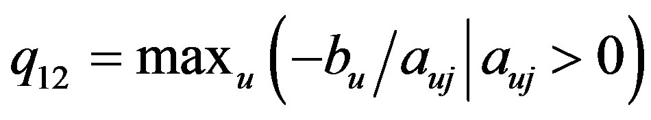
Let us consider a simple algorithm to estimate dependence degree of some non-homogeneous inequalities in the BSM containing only independent inequalities. Let us compute and put in order of increasing the  values for all
  for each column variable
 . Assume the first place in this list is occupied by the row (several rows) corresponding to the
 , variable and the second—to the
  variable. (In the case, when
 , we proceed to the next column variable). If we make the JE with the
  resolvent element, we will find that the
  constant term is negative. With
  increase by the
  value the
  inequality would be found out dependent of the second kind. It follows that
 .
.
Proposition 3.3. If  and no negative coefficients are found out among the u-th row coefficients, this inequality can be considered to be “almost dependent” and it can be eliminated from the BSM. Similar computation cycles should be repeated, the pattern of column variables should be changed every time.
3.7. Inequalities Number Expansion Process Control with Variables Elimination by CAC
While using matrix additional cleanup it is possible to find a simple trade-off between two contradictory stimuli: the desire to prevent too rapid number expansion of the inequalities defining projections and the desire to prevent polyhedron surface excessive alteration. To implement such a trade-off let us assume two parameters.
The first one is represented as the  inequalities coarsening maximum admissible rate in the course of matrix additional cleanup and therewith associated the “working value”
  of this rate, where the
  controlled variable can take the discrete values 0,1,2,···,9,10. For practical use it is reasonable to assume the
  value to be within the range of 0.05 - 0.10.
The second parameter is the maximum admissible multiplicity  of row number in the matrix increase with elimination of variables in respect of the parent matrix. Thus inequalities number admissible threshold valueв is
 . The
. The  rational value depends on the available “computation resources” and can vary within 3 - 10.
Let us assume that after the elimination of the next variable  the working value
 , and the number of inequalities in the matrix is
 . Assume that after the elimination of the variable xk+1 with the help of FCA algorithm and the complete cleanup of matrix the inequalities number therein exceeds the preset threshold. In this case let us additionally clean the matrix with the ek rate. If it doesn’t provide the rk+1 value decrease needed, let us assume
 , then let us again additionally clean the matrix, but now in an “intense mode”, i.e. with the ek+1 rate. Let us repeat this procedure until one of the two conditions is fulfilled:
1)  and
and , or 2)
  and
and .
.
In the first case it will be possible to further intensify matrix cleanup restricting inequalities number in newly generated matrices during the following iterations if necessary. In the second case the process of variable elimination with complete and additional cleanup of generated matrices will be continued, however, the possibility of matrix additional cleanup intensification will be lost.
If in the course of variable elimination it is necessary to resort to matrix additional cleanup, then not only the corresponding matrix is compared to each  -th iteration, but also the ek coarsening rate value, which was used during its generation. It makes it possible to avoid inadmissible solutions occurring as a result of the polyhedron “improper” extension during “descent of matrix pyramid”. Precisely, in the formally computable range of the
  -th variable
  it is permissible to chose xk values only in the range
 , where
4. Stability of the Polyhedron Orthogonal Projection and Complexity of Its Algorithm
4.1. Stability of the POP Algorithm
Let us give an inequality system (4). It gives us a compact polyhedron . Here two cases are possible:
  is solid or singular. In the first case it is valid.
Proposition 4.1. If the polyhedron  is solid, then POP is stable.
Proof. Using (4), we introduce M = maxi max . Denote by
  such a perturbation of inequality
 , in which all coefficients
  and free member
  have an increment in absolute value not exceeding a given
 . Denote by
  the polyhedron obtained if in (4) inequalities
  replaced by
 . Suppose that
  is the face in
  and
and —in
—in  asked by the conditions
  and
and , respectively. For an inequality
  we introduce the rate
 . Suppose that all inequalities have nonzero rates. Define
 . We fix
and take . Then we have
It follows that . We now take
 . Then we have
 . Hence
 . Note that
 Immediately it is verified that there exists
  such that with condition
  for any
 it is valid:
  It follows that
 . Here
  is the distance from the point to the space.
Similarly, it is easy to see that . Denote by
 —neighborhood of
 . Then we have
 . (6)
. (6)
Denote by  the orthogonal projection on a subspace. Since the distance between the points cannot increase in the projection, from (6) it follows that
 (7)
(7)
From (7) it follows that a sufficiently small perturbation of coefficients and free members of inequalities leads to a small perturbation of polyhedron projection. This completes the proof.
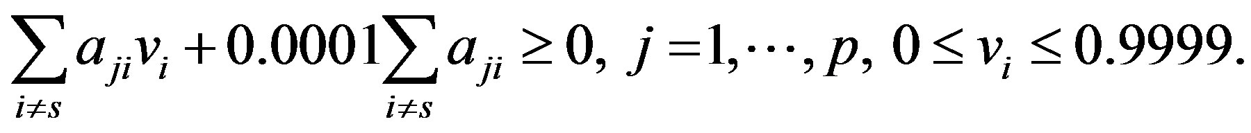
In the case of singular polyhedron an arbitrary small perturbation can lead to a significant change in projection as follows Example 4.1. Let  be the polyhedron defined by the inequalities:
 .
.
Denote by  the orthogonal projection on the axis
 . We introduce a perturbation
  of
of .
.
 .
.
Then we have  and for any
  it holds
 .
.
4.2. The Complexity of the POP Algorithm
The complexity of POP algorithm is defined by two factors:
1) the growth of inequality number in the system by iterations;
2) the complexity of the algorithm of redundant inequality cleanup for a single iteration.
Let us consider 1). Let  be a compact polyhedron defined by the inequality system (4) and
  be the orthogonal projection onto a subspace
 . Note that single iteration of the orthogonal projection procedure is accompanied by a full cleanup of redundant inequalities. Therefore, an inequality
  in the system of projection corresponds to hyperplane
  containing a face
  of
of . Similar to [16,17] this hyperplane can be represented as
  projection of the intersection of
  hyperplanes
  of the original inequality system. Hence, we obtain an estimation of the number
  of inequalities for this projection by the binomial coefficients:
 . (8)
. (8)
Here  is the number of inequalities (lj) in (4) and
  correspond to parallelepiped restrictions.
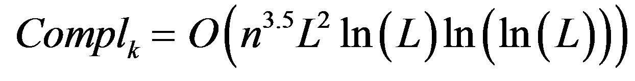
At 2) we estimate the cause of complexity of redundant inequality cleanup. It is determined by the number of appeals to the solution of linear problems (5). Typically this problem has a low dimension and is solved by means of the simplex-algorithm. As it is well known the simplex-algorithm has an exponential complexity [18]. Note that in the linear problem (5) the threshold  of accuracy of its solution is introduced. This allows the use of the polynomial algorithms of linear problem solution. Here Khachiyan [19] and Karmarkar [20] algorithms are known. The Karmarkar algorithm [20] is more efficient and has the complexity
 .
.
Here  is the number of free variables of linear problem and
  is the number of bits of input to the algorithm. It is suggested that a linear problem is solved for each inequality. Then for complexity
  of the redundant inequality cleanup of the iteration
 , we have the majorant
 . (9)
. (9)
5. Computational Experiment Results
In accordance with the considered algorithm we have developed a demonstration version of the program implementing the orthogonal projecting procedure (OPP) by using the language VISUAL BASIC 6th version with a 32-bit compiler. During computational experiments the following computer resources were used: PC Intel-Core2 with clock speed of 2.67 GHz, capacity of internal memory of 3.25 Gb and the operating system Microsoft Windows XP Professional 2003. The computational experiments aimed to analyse FCA improvement proposed measures effectiveness. The matrices of form (3) were investigated. The LP problem was used for computation accuracy strict check with OPP implementation. In particular, first the projection of the entire feasibility region is constructed on the objective function axis. Then, the optimal resolution vector is determined with the previously computed matrices sequence “descent”. This estimation of solution accuracy is made by its comparison with the same problem solving by means of simplex-method. Herewith material inconsistency is admissible only in the case, if the problems pair being considered has an ambiguous solution.
When the procedure is used in practice, the following parameters are rather essential beyond computational accuracy: 1) expansion maximum degree of the number of inequalities with the elimination of variables; 2) computing time needed for the elimination of a given set of variables. This time depends on available computation resources, the specific nature of the parent matrix, the number of eliminated variables and after all on the algorithm being used. Therefore, all experiments were held on the same computer, with the same structure matrices (3), with the same requirement of all nonbasic variables elimination. The matrices being considered had only various  dimensions of polyhedra. Herewith the parent matrix contains
  rows, since
  rows are supplemented by the requirements
 . Matrices inadmissible expansion with the use of FCA only is clearly illustrated in Table 1 with
 . At the next stage algorithm performance capabilities were investigated with complete cleanup of matrices, but without additional cleanup, in particular, without their expansion control. At the final stage the algorithm with additional cleanup, i.e. with “coarsening” was considered.
Table 3 gives the consolidated results of numerical experiments for various dimensions of the parent matrices. The Table 3 contains N—parent matrix dimensionsM—inequalities in the matrix number maximum expansion after its complete cleanupT—time (sec) of all variables eliminationRelative deviations from the simplex solution of the LP appropriate problem:
D1—deviation of the optimal value of the objective function;
D2—maximum deviation of the optimal solution variables;
D3—average deviation of the optimal solution variables.
All Table 3 rows (excluding the last two rows) reproduce results of convolution with the use of matrix complete cleanup, but without coarsening. With matrices cleanup in LP problems, which are represented in the last two rows, a coarsening with threshold 3 and maximum rate 0.1 for  and 0.12 for
  was used. The Table 3 analysis shows, that the rate-determining
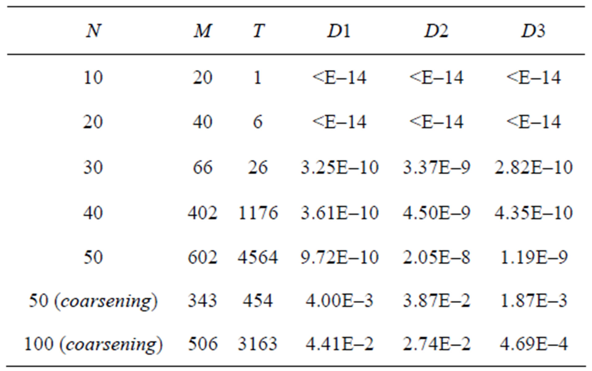
Table 3. Combined results of experiments.
factor with convolution of the high-dimensional inequality systems is not so much expansion thereof, as computation time. In the above mentioned conditions the admissible computation amount (76 min 4 sec) was obtained with  with the use of only matrix complete cleanup. The fragments of corresponding automatically generated protocol, giving the idea about inequality system convolution history, are represented in Table 4.
Table 4 illustrates the fact that the generated matrix cardinality dependence on the next iteration index is ambiguous. It is determined by the variables elimination order and by the distribution of positive and negative coefficients in the eliminated column.
Comparison of the data represented in the two rows of Table 3 for problem with  dramatizes matrix additional cleanup algorithm (coarsening algorithm) performance capabilities. In the discussed example its use made it possible to reduce inequality system maximum expansion by 1.76 times, computation time—by 10.05 times, however, it is accompanied by objective function optimal value computation accuracy loss up to the level of 0.004. In those cases, when such loss is admissible, the use of the coarsening algorithm can be considered to be rather effective. Below the algorithm of choosing the of attractive admissible point 3.3 is illustrated in example
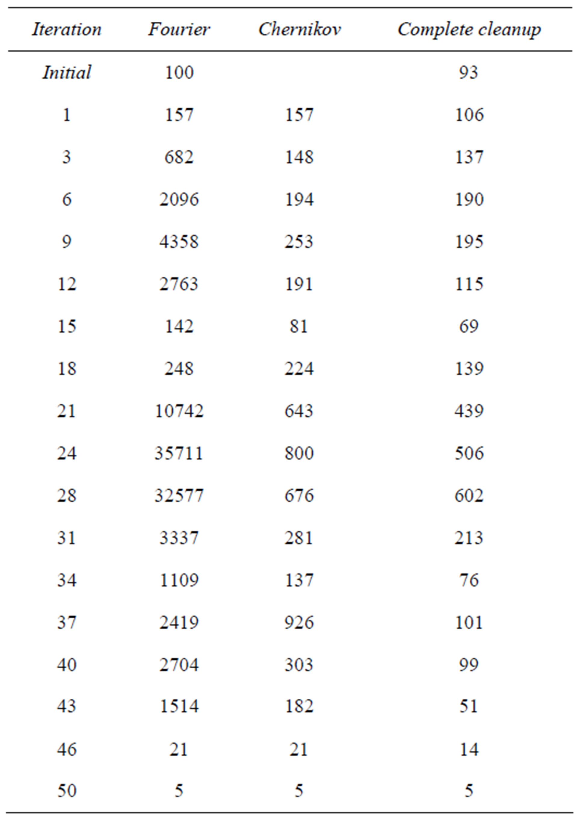
Table 4. Convolution history for N = 50.
(3) with . The course of building of system (3) solution in the explicit form is given in Table 5. Note that the value of variable 1 is calculated, i.e. it is not given in the dialog.
6. Conclusions
The computer experiments performed enable us to establish the following:
Ÿ The algorithms of matrix complete cleanup make it possible to obtain quite a high accuracy of computation.
Ÿ A rapid increase in computation time span with problem dimensions increase is the main disadvantage of the demonstration version of the program used.
Ÿ The use of matrix additional cleanup is effective in cases, where the initial information is in error of several percents.
Ÿ We can hope that estimations (8), (9) of the complexity of POP are overvalued and can be improved significantly.
It is useful to mention the following trends of OPP use in applied research:
In defining linear model of an object whose variables are not relevant for the investigator, though they cannot be neglected, the corresponding set projection to subspace, not containing those variables, will make it possible to retain all the features of the model being investigated. Such an application of the convolution method is known
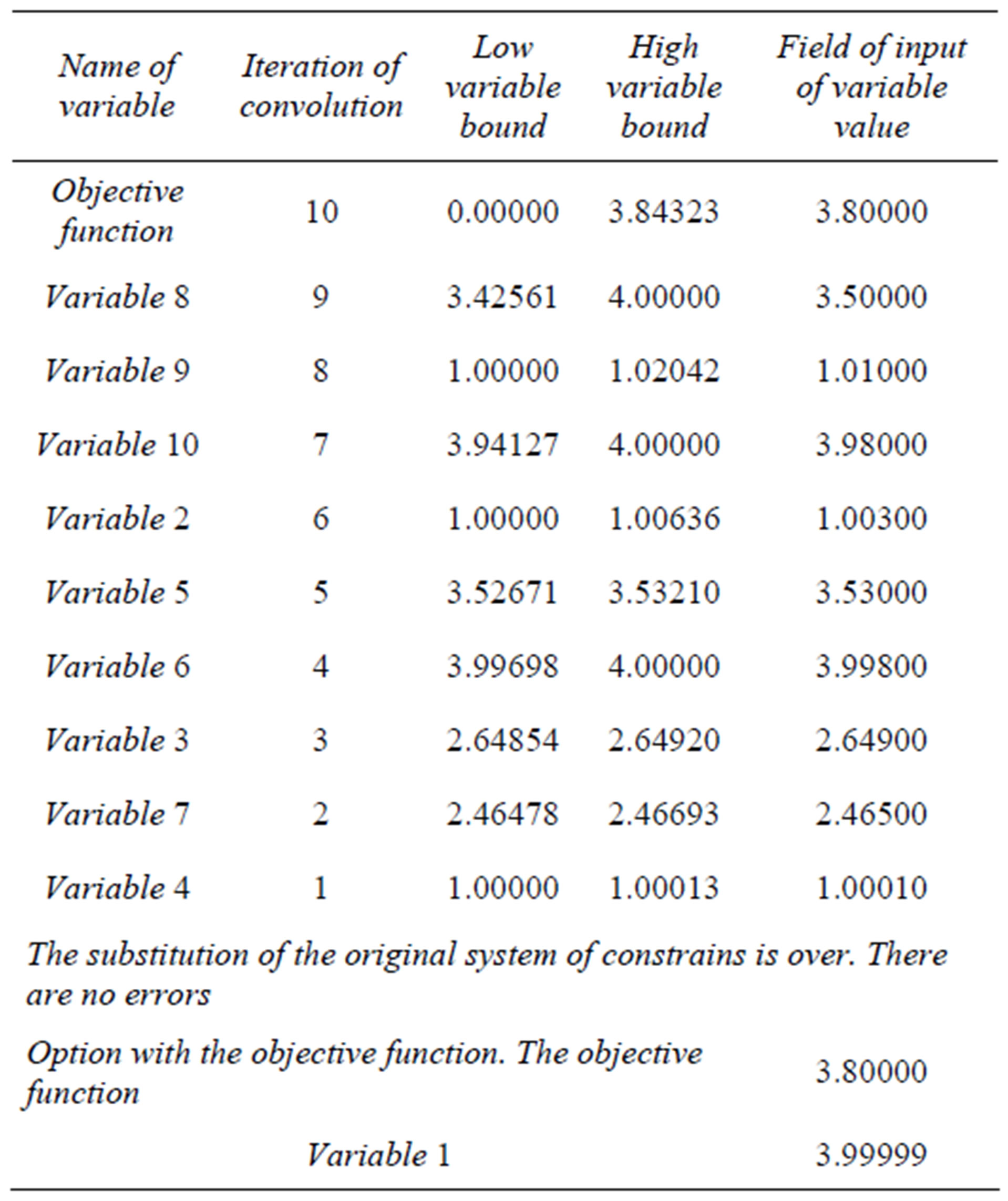
Table 5. Dialog interface for the building of an inequality system solution.
in biophysics (Nikolaev, Burgard and Maranas [21]).
In parametric programming problems, in which it is useful to find the dependence of LP problem optimal solution on such linear model parameters as absolute terms of constrains and (or) boundaries of variables (Keerthi and Sridharan [22]).
In the problems of process-admissible deviations from any products rated values, for which operability scope thereof  is defined by a linear model. The use of OPP will make it possible use
  much more fully with a transfer from universally accepted mutually independent tolerances to a system of dependent tolerances, because it allows us to replace a parallelepiped inscribed in
  with a polyhedron.
In various problems on agreeing solutions in search of a compromise between partners (Shapot and Lukatskii [7]).
In problems of a multi-objective choice while projecting region of feasibility on subspace of criteria (Karbovsky, Lukatskii and Shapot [23]).
7. Acknowledgements
The authors are grateful to the referees for their useful comments.
REFERENCES
- J. B. Fourier, “Solution d’une Question Particulière du Calcul des Inégalités,” Nouvean Bulletin des Sciences par la Société Philomatique de Paris, 1826, p. 99.
- D. V. Shapot, “On the Construction of Orthogonal Projections of Point Sets Defined by a System of Inequalities,” Journal Computational Mathematics and Mathematical Physics, Vol. 11, 1971, pp. 1113-1126.
- S. N. Chernikov, “Linear Inequalities,” Nauka, Мoscow, 1968.
- V. A. Bushenkov and A. V. Lotov, “An Algorithm for Analysis of Inequality Dependences in a Linear System,” Journal Computational Mathematics and Mathematical Physics, Vol. 20, 1980, pp. 562-572.
- A. V. Lotov, “On the Estimate of Stability and the Condition Number of the Solution Set of a System of Linear Inequalities,” Journal Computational Mathematics and Mathematical Physics, Vol. 24, 1984, pp. 1763-1774.
- I. I. Eremin and A. A. Makhnev, “International Workshop on Algebra and Linear Optimization Dedicated to the 90th Anniversary of the Birth of S. N. Chernikov,” Ural State University Bulletin, Vol. 30, 2004, pp. 183-184.
- D. V. Shapot and A. M. Lukatskii, “A Constructive Algorithm for Foldind Large-Scale Systems of Linear Inequalities,” Computational Mathematics and Mathematical Physics, Vol. 48, No. 7, 2008, pp. 1100-1112. doi:10.1134/S0965542508070038
- T. S. Motzkin, H. Raiffa, G. L. Thompson and R. M. Trall, “The Double Description Method,” Contributions to the Theory of Games, Vol. 2, 1953, pp. 51-73.
- F. P. Preparata and M. I. Shamos, “Computational Geometry. An Introduction,” Springer-Verlag, Berlin, Heidelberg, New York, Tokyo, 1985.
- V. N. Shevchenko and D. V. Gruzdev, “Modifications of Fourier-Motskin Algorithm for Triangulation Construction,” Discrete Analysis and Investigation of Operations, Series 2, Vol. 10, 2003, pp. 53-64.
- R. V. Efremov, G. K. Kamenev and A. V. Lotov, “Constructing an Economical Description of a Polytop Using the Duality Theory of Convex Sets,” Doklady Mathematics, Vol. 70, 2004, pp. 934-936.
- A. I. Golikov and Y. G. Evtushenko, “A New Method for Solving Systems of Linear Equalities and Inequalities,” Doklady Mathematics, Vol. 64, 2001, pp. 370-373.
- P. O. Gutman and I. Ioslovich, “On the Generalized Wolf Problem: Preliminary Analysis of Nonnegativity of Large Linear Programs Subject to Group Constrains,” Automation Telemech, No. 8, 2007, pp. 116-125.
- S. Paulraj and P. Sumathi, “A Comparative Study of Redundant Constrains Identification Methods in Linear Programming Problems,” Mathematical Problems in Engineering, Vol. 2010, 2010, pp. 1-16. doi:10.1155/2010/723402
- D. V. Shapot and A. M. Lukatskii, “A Constructive Algorithm for Building Orthogonal Projections of Polyhedral Sets,” Optimization, Control, Intelligence, Sibirian Energy Institute, Irkutsk, 1995, pp. 77-91.
- D. Hilbert and S. Cohn-Fossen, “Anshauliche Geometrie,” Verlag J. Springer, Berlin, 1932.
- A. D. Alexandrov, “Convex Polyhedra,” Springer-Verlag, Berlin, 2005.
- V. Klee and G. Minty, “How Good Is the Simplex-Algorithm,” Proceedings of the Third Symposium on Inequalities, Los Angeles, 1972, pp. 159-175.
- L. Khachiyan, “A Polynomial Algorithm in Linear Programming,” Soviet Mathematics—Doklady, Vol. 20, 1979, pp. 191-194.
- N. Karmarkar, “A New Polinomial Time Algorithm for Linear Programming,” Combinatorics, Vol. 4, No. 4, 1984, pp. 373-395. doi:10.1007/BF02579150
- E. V. Nikolaev, A. P. Burgard and C. D. Maranas, “Education and Structural Analysis of Concerved Pools for Genom-Scale Metabolic Reconstruction,” Biophysical Journal, Vol. 88, No. 1, 2005, pp. 37-49. doi:10.1529/biophysj.104.043489
- S. S. Keerthi and K. Sridharan, “Solution of Parametrized Linear Inequalities by Fourier Elimination and Its Applications,” Journal of Optimization Theory and Applications, Vol. 65, 1990, pp. 161-169.
- I. N. Karbovsky, A. M. Lukatskii and D. V. Shapot, “Use of Orthogonal Projection Method by the Example of Analysis of Industries Possible Price Response to Natural Monopolies Products Price Shocks,” Proceeding of the Second International Conference MLSD 2008, Institute of Control Sciences, Moscow, 2008, pp. 117-126.
NOTES
*Corresponding author.